I have a term of art for a lot of the survey research that is shared with me from my clients: a “hit-and-run.” A hit-and-run happens when researchers do a study on behalf of a client, tab the results, make pretty charts and graphs, then exit the building with the decision-maker wondering what they’re supposed to do next. They happen when the findings report remains at the surface level of simply describing the results from each question asked, but not considering if any of those questions exist within a relationship that could be useful.
You can describe your data in extraordinary detail–means, distributions, cross-tabs, cluster profiles–and still not answer the question a decision-maker most wants answered: What can I do to change or act on any of this? Does perceived trustworthiness influence endorsement potential? Does relatability matter more than competence? Which of the things you measured is the one that moves the needle?
Answering that requires you to look at relationships between variables. Two tools get you there: correlation and regression. Both are accessible, both work well with survey data, and both are directly useful for the kind of analysis your teams are doing right now.
Start with Correlation
A correlation coefficient (r) measures the strength and direction of a linear relationship between two variables. It ranges from −1 to +1. A value near +1 means the variables move together; near −1 means they move in opposite directions; near 0 means there’s no linear relationship to speak of.
In survey research, you’ll use correlation constantly. Do respondents who rate a celebrity as trustworthy also see her as a strong endorser? Do people who find her relatable also think she does meaningful work? A correlation matrix gives you a quick, honest first pass through your data.
That matrix tells you which pairs of variables are associated and how strongly. It’s often enough to answer early-stage research questions. But correlation has a ceiling. It tells you that two variables are related. It doesn’t tell you how much one changes when the other moves by a unit. It treats both variables symmetrically, with no distinction between the thing doing the influencing and the thing being influenced. And it can’t tell you how much of the variation in your outcome a given predictor explains.
When you’re asking whether X influences Y, not just whether they’re correlated, you need regression.
When You Need More Than Correlation
Simple linear regression takes the same linear relationship and adds direction. You specify an outcome (the thing you’re trying to explain) and a predictor (the thing you think influences it). In return, you get three things correlation cannot provide.
A coefficient tells you the expected change in the outcome for a one-unit increase in the predictor. If the coefficient for trustworthiness on endorsement potential is 0.7, that means each one-point increase in perceived trustworthiness is associated with a 0.7-point increase in endorsement potential.
R² tells you the proportion of variance in the outcome that the predictor explains. Think of it as a measure of explanatory power. An R² of 0.15 means your predictor accounts for 15% of the variation (real but modest). An R² of 0.45 means you’ve captured nearly half the story.
A p-value tells you whether the relationship is statistically distinguishable from zero. The conventional threshold is p < 0.05, but remember that statistical significance and practical significance are different things. A predictor can be significant and still explain very little. Also, the p < 0.05 threshold was invented by academics. Many models in the real world of marketing are considered valid with p < 0.10.
Here’s the payoff. You can run separate regressions for each predictor and compare them side by side:
Code
predictors <-c("atts_relatable", "atts_meaningful_work","atts_trustworthy", "atts_competent")results <- predictors |>set_names() |>map(\(var) lm(reformulate(var, "talent_endorse"), data = df)) |>map_dfr(\(mod) {bind_cols(tidy(mod) |>filter(term !="(Intercept)") |>select(term, estimate, p.value),glance(mod) |>select(r.squared) ) })results |>gt() |>tab_header(title ="Simple Linear Regressions on Endorsement Potential",subtitle ="Each row is a separate model with a single predictor" ) |>tab_options(table.align ="left" ) |>opt_row_striping(row_striping =TRUE) |>fmt_number(columns =where(is.numeric),decimals =2 )
Simple Linear Regressions on Endorsement Potential
Each row is a separate model with a single predictor
term
estimate
p.value
r.squared
atts_relatable
0.40
0.00
0.34
atts_meaningful_work
0.39
0.00
0.29
atts_trustworthy
0.42
0.00
0.35
atts_competent
0.42
0.00
0.32
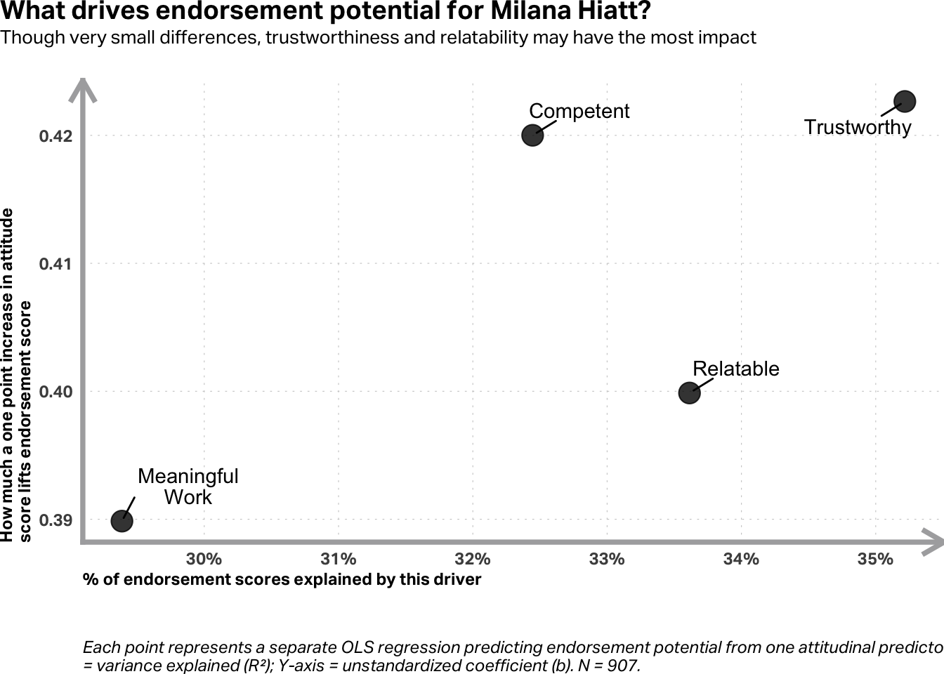
This produces a table with each predictor’s coefficient, p-value, and R². Now you can answer the question you started with: which attribute matters most? The predictor with the largest R² explains the most variation in endorsement potential. The one with the largest coefficient moves the outcome the most per unit. These two rankings often agree, but not always.
Code
endorse_driver_caption <-str_glue("Each point represents a separate OLS regression predicting endorsement potential ","from one attitudinal predictor. ","X-axis = variance explained (R²); Y-axis = unstandardized coefficient (b). N = {nrow(df)}.")# Add clean labels for the plotresults <- results |>mutate(label =case_when( term =="atts_relatable"~"Relatable", term =="atts_meaningful_work"~"Meaningful Work", term =="atts_trustworthy"~"Trustworthy", term =="atts_competent"~"Competent" ))results |>ggplot(aes(x = r.squared, y = estimate)) +geom_point(size =5, alpha =0.8) + ggrepel::geom_text_repel(aes(label =str_wrap(label, 12)),box.padding =0.6, point.padding =0.25, lineheight =0.85 ) +scale_x_continuous(labels =percent_format(accuracy =1)) +theme(plot.margin =margin(0, 0, 0, 0),axis.line.x =element_line(color ="#acacae",linewidth =1.3,arrow =arrow(ends ="last", length =unit(12, "pt")),lineend ="square" ),axis.line.y =element_line(color ="#acacae",linewidth =1.3,arrow =arrow(ends ="last", length =unit(12, "pt")),lineend ="square" ),axis.title.x =element_text(hjust =0, face ="bold"),axis.title.y =element_text(hjust =0, face ="bold"),axis.text.x =element_text(size =9, face ="bold"),axis.text.y =element_text(size =9, face ="bold"),panel.grid.minor =element_blank(),panel.grid.major =element_line(linetype ="dotted"),plot.caption =element_text(hjust =0, margin =margin(t =28, unit ="pt")),plot.title =element_text(size =14, margin =margin(t =0, b =0, unit ="pt")),plot.title.position ="plot",plot.subtitle =element_text(margin =margin(t =3, b =18, unit ="pt"), size =10) ) +labs(title ="What drives endorsement potential for Milana Hiatt?",subtitle ="Though very small differences, trustworthiness and relatability may have the most impact",x ="% of endorsement scores explained by this driver",y =str_wrap("How much a one point increase in attitude score lifts endorsement score", 45),caption =str_wrap(endorse_driver_caption, 120) )
In a recent study for a technology services company, we used exactly this approach to compare how much credibility and commitment each influenced customers’ intent to renew. Both were statistically significant. But commitment explained substantially more variance in intent–a finding that redirected where the company focused its retention efforts. The table of coefficients and R² values made the case in two rows.
A Few Cautions
Regression with survey data is powerful but not magic. A few things worth keeping in mind.
Correlation still isn’t causation.
Regression tells you that X and Y move together in a specific, directional way. It doesn’t prove that changing X will change Y. For causal claims, you need an experiment. We’ll cover that soon enough in the course.
Likert scales are imperfect predictors.
A five-point or seven-point scale gives you limited variance to work with. R² values in survey research are often lower than you’d see with continuous behavioral data. That’s normal. Don’t let a modest R² convince you the finding is useless.
One predictor at a time is a starting point, not a destination.
The approach above (running separate simple regressions) is a clean way to explore which variables matter individually. But your predictors are correlated with each other. Respondents who rate a celebrity as trustworthy probably also rate her as competent. Multiple regression, which includes several predictors simultaneously, lets you see which ones matter after controlling for the others. We’ll get there.
AI Exploration Prompts
“I have a survey dataset with several Likert-scale attitude variables and a single outcome variable measuring endorsement potential. Walk me through running a correlation matrix and then simple linear regressions for each predictor in R.”
“I ran two simple regressions. One has R² = 0.25 and the other has R² = 0.08. Both are significant. Help me explain to a non-technical audience what this means for which variable matters more.”
“What’s the difference between a correlation coefficient and a regression coefficient? When would I report one versus the other?”