| variable | N | Median | Mean | SD | Min | Max |
|---|---|---|---|---|---|---|
| aff1 | 500 | 5 | 4.70 | 1.27 | 1 | 7 |
| aff2 | 500 | 5 | 4.57 | 1.31 | 1 | 7 |
| aff3 | 500 | 5 | 4.79 | 1.27 | 1 | 7 |
| beh1 | 500 | 4 | 4.19 | 1.37 | 1 | 7 |
| beh2 | 500 | 4 | 4.02 | 1.35 | 1 | 7 |
| beh3 | 500 | 4 | 4.26 | 1.38 | 1 | 7 |
| int1 | 500 | 4 | 4.50 | 1.30 | 1 | 7 |
| int2 | 500 | 4 | 4.33 | 1.30 | 1 | 7 |
| int3 | 500 | 5 | 4.53 | 1.30 | 1 | 7 |
| sens1 | 500 | 5 | 4.84 | 1.33 | 1 | 7 |
| sens2 | 500 | 5 | 4.59 | 1.35 | 1 | 7 |
| sens3 | 500 | 5 | 4.53 | 1.35 | 1 | 7 |
Analyzing Factors
Lecture
Measuring and analyzing latent variables in survey datasets.
Presented by:
Larry Vincent,
Professor of the Practice
Marketing
Larry Vincent,
Professor of the Practice
Marketing
Presented to:
MKT 512
April 21, 2026
MKT 512
April 21, 2026

From scales to factors…
A galaxy is like a factor in the universe.
Factor analysis
- Identify clusters of inter-correlated variables
- Family of multivariate statistical techniques for exploring correlations between variables
- Empirical approach to test theoretical data structures
- Widely used method in psychometric instrument development
Purposes
- Data reduction
Reduce number of variables in dataset to smaller set of factors - Theory development
Detect structural relationships between variables, often latent structures that describe a governing force
Theory development
- Investigate underlying correlation patterns shared by variables in order to test a theoretical model (i.e. How many personality factors are there?)
- Done well, always addresses a theoretical question
(rather than just calculating an arbirtrary factor score)
Factors in the wild
Approcahes to factor analysis
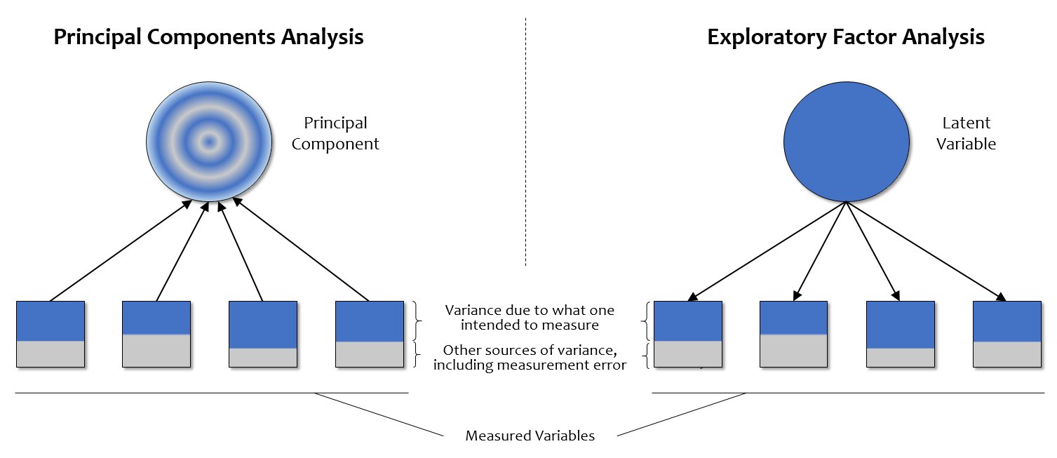
- Principal Components Analysis (PCA)
A data reduction technique that summarizes variance in observed variables without assuming underlying latent constructs. Often used as a first step to explore structure and simplify data - Exploratory Factor Analysis (EFA)
Explore and summarize underlying correlational structure for a dataset - Confirmatory Factor Analysis (CFA)
Tests that a correlational structure, as hypothesized, exists in a dataset and measures “goodness of fit.”
Differences
Assumptions
- Garbage in; Garbage Out
- Sample size matters
(Min = >5 cases per variable; Ideal = >20 cases per variable) - Interval or ratio data suitable for correlation analysis
- Normality: normal distribution is ideal but not required
- Outliers: Factor analysis is sensitive to outliers, which should be removed or transformed
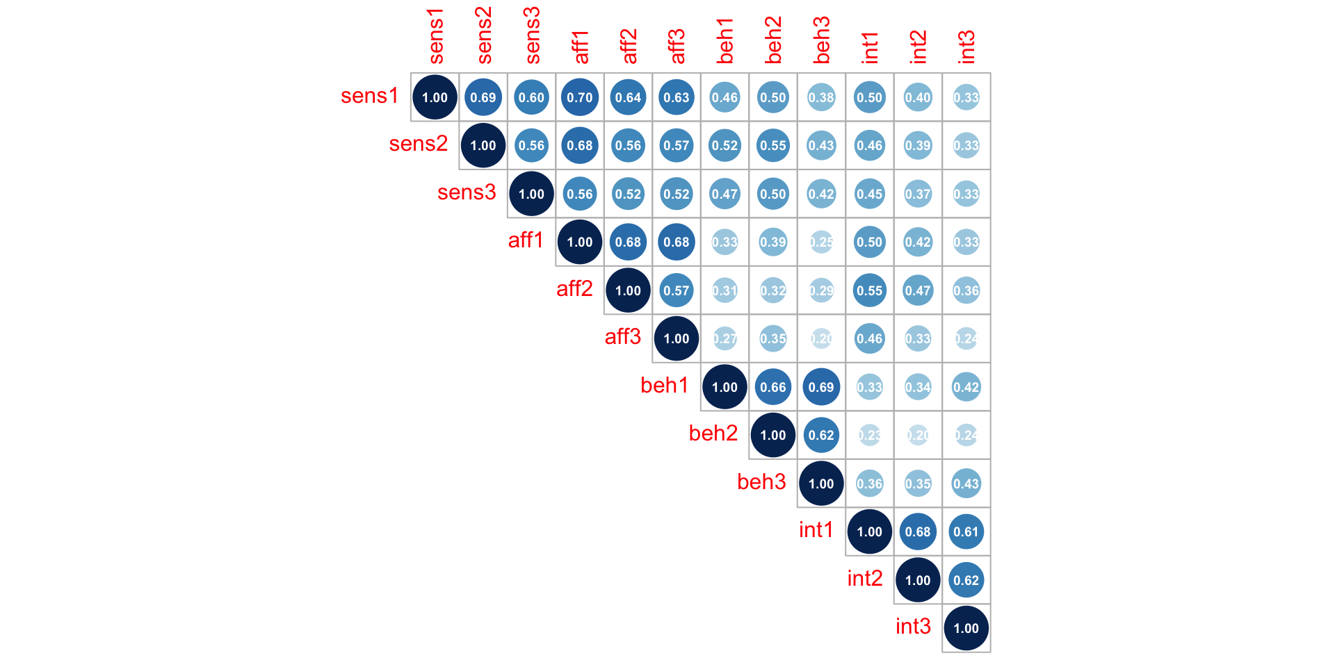
- Requires strong evidence of correlation
(correlation matrix coefficients > 0.3)
Two ways to use factor analysis
Discovery
What structure is in this data?
- Test assumptions
- Select type of factor analysis
- Determine number of factors
- Select items
- Name and define factors
- Examine correlations among factors
- Analyze internal reliability
- Compute composite scores
Validation
Does this data support the hypothesized model?
- Specify the hypothesized model
- Test assumptions
- Fit the factor structure
- Evaluate loadings and cross-loadings
- Assess subscale reliability
- Examine factor correlations
- Judge fit — accept, revise, or reject
- Compute composite scores
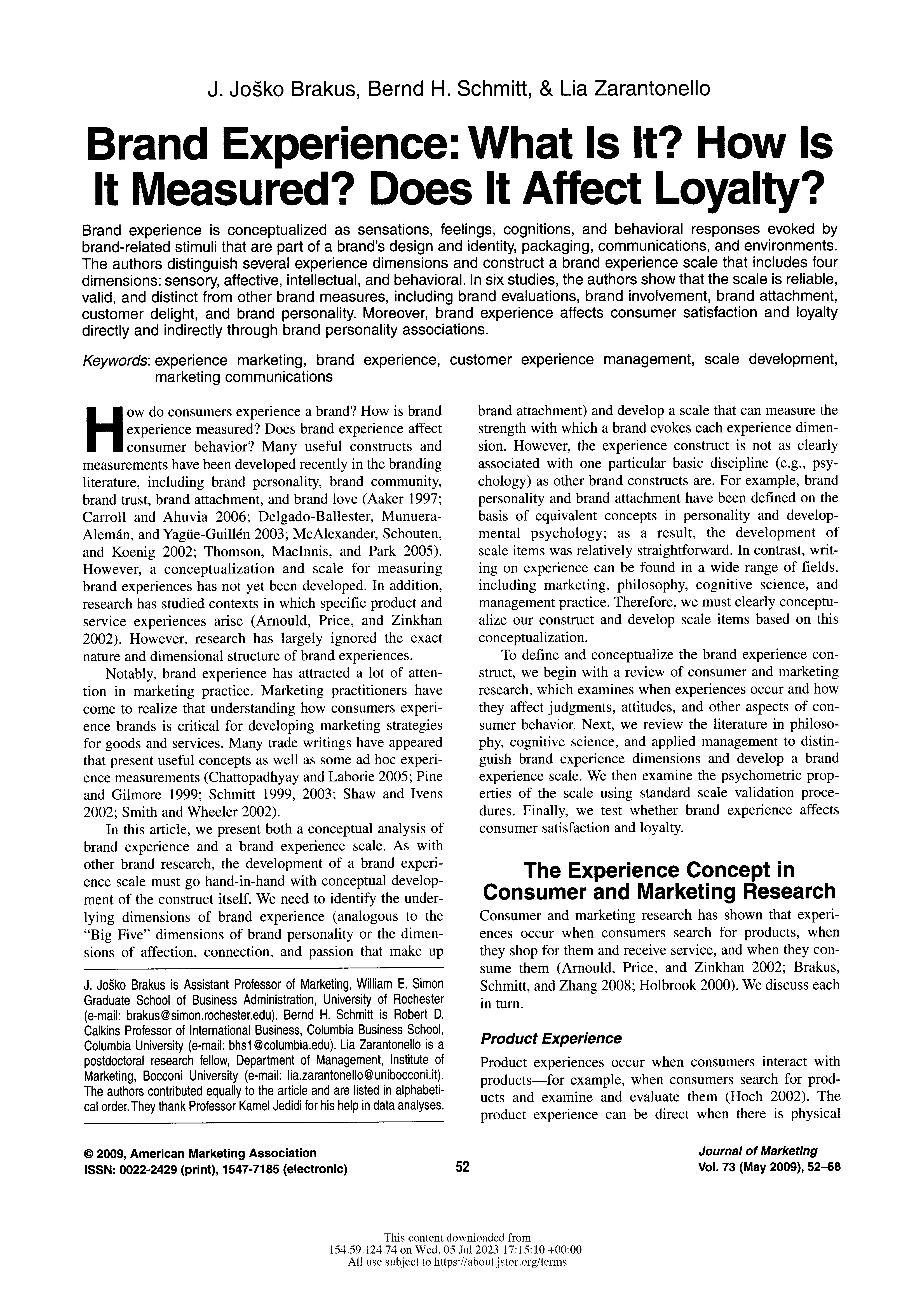
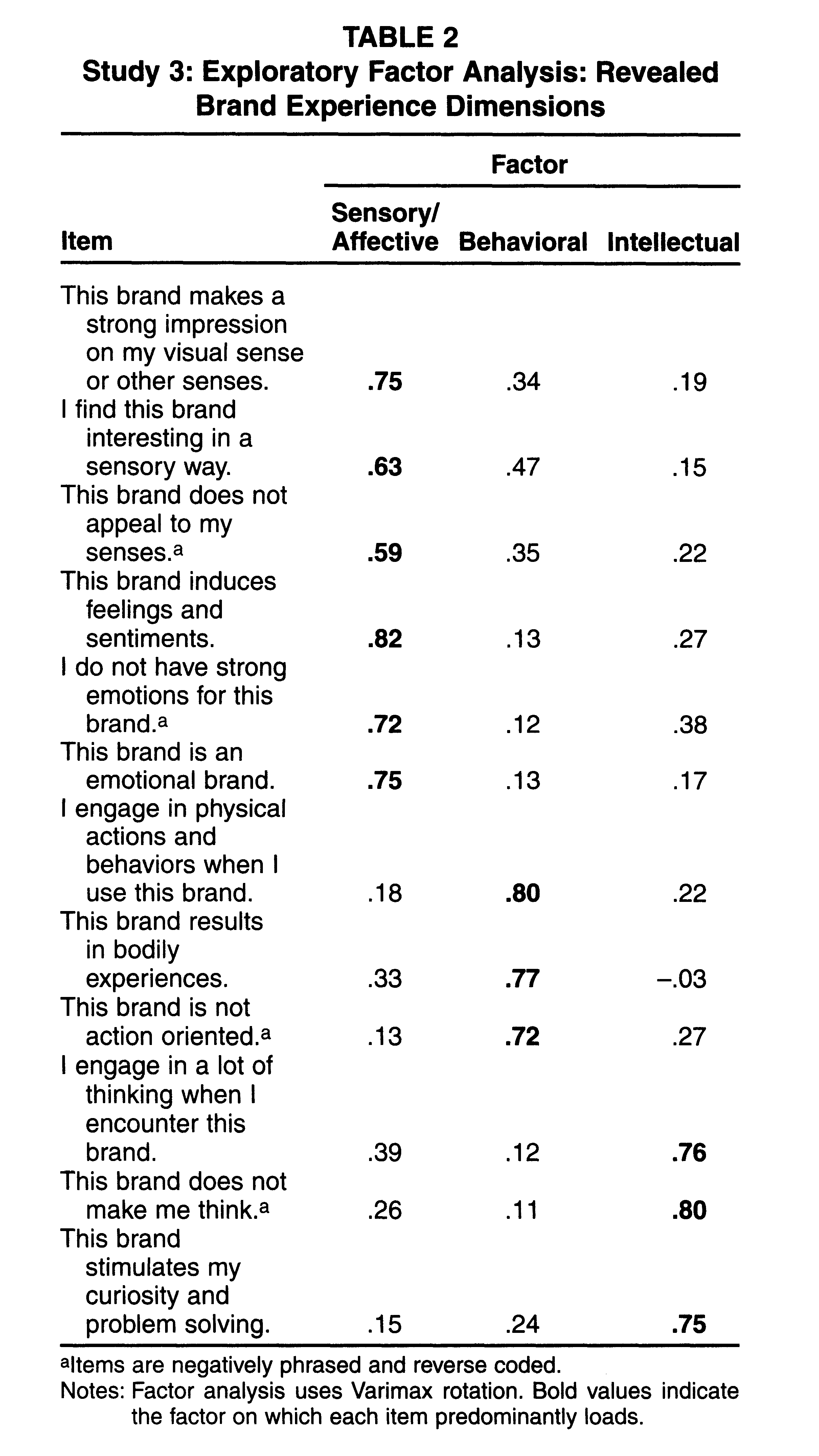
The Brand Experience scale
| Factor | Column | Statement |
|---|---|---|
| Sensory/Affective | sens1 | This brand makes a strong impression on my visual sense or other senses. |
| sens2 | I find this brand interesting in a sensory way. | |
| sens3 | This brand does not appeal to my senses. (r) | |
| aff1 | This brand induces feelings and sentiments. | |
| aff2 | I do not have strong emotions for this brand. (r) | |
| aff3 | This brand is an emotional brand. | |
| Behavioral | beh1 | I engage in physical actions and behaviors when I use this brand. |
| beh2 | This brand results in bodily experiences. | |
| beh3 | This brand is not action oriented. (r) | |
| Intellectual | int1 | I engage in a lot of thinking when I encounter this brand. |
| int2 | This brand does not make me think. (r) | |
| int3 | This brand stimulates my curiosity and problem solving. |
(r) = reverse-scored before analysis
Source: Brakus, Schmitt & Zarantonello (2009), Journal of Marketing 73(3), 52–68.
Brand experience dataset
Correlations
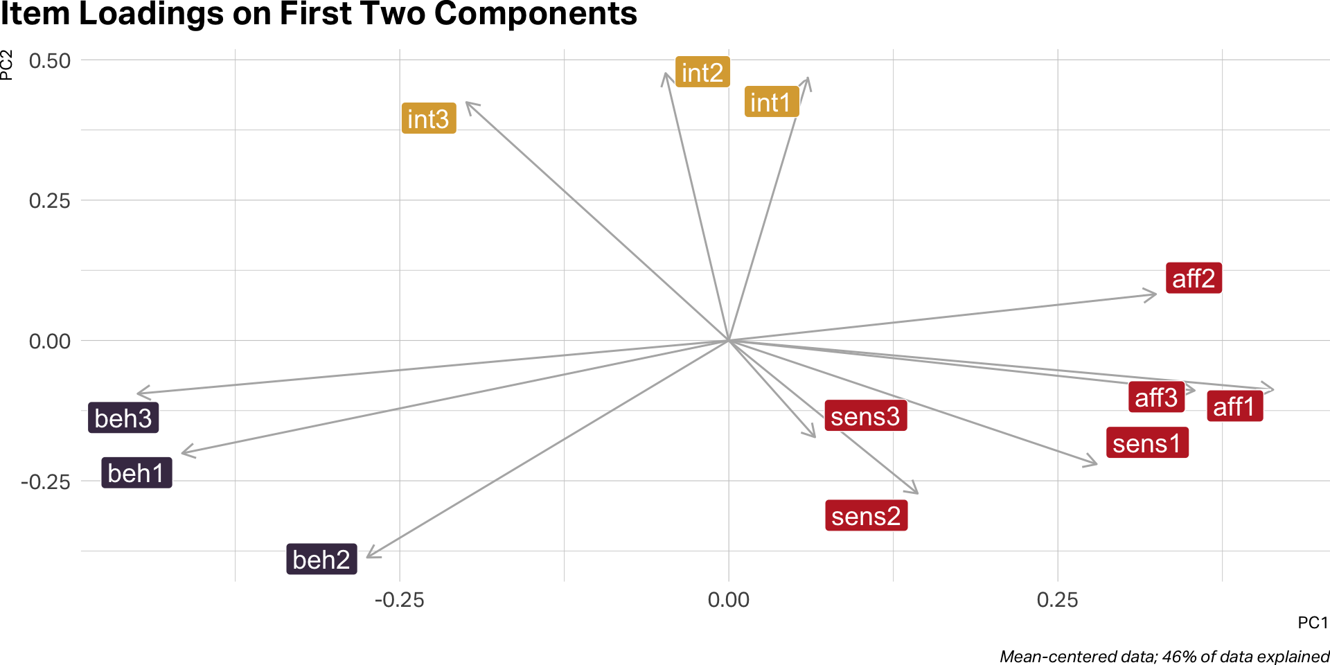
What is Principal Component Analysis?
PCA
PCA in R
# Generate PCA data for the value attributes
atts_pca <- prcomp(atts, scale. = TRUE)

# Extract the component variables from the rotation matrix
atts_pca_tidy <- tidy(atts_pca, matrix = "rotation")

# Add the component data back to our original datafram for easy analysis
atts_pca_augment <- augment(atts_pca, atts)
Rows: 500
Columns: 25
$ .rownames <chr> "1", "2", "3", "4", "5", "6", "7", "8", "9", "10", "11", "…
$ sens1 <dbl> 7, 5, 6, 5, 2, 5, 3, 3, 4, 4, 4, 4, 2, 4, 3, 4, 5, 4, 4, 4…
$ sens2 <dbl> 6, 4, 5, 7, 4, 6, 4, 4, 4, 4, 3, 4, 3, 4, 3, 5, 5, 3, 4, 4…
$ sens3 <dbl> 6, 5, 6, 7, 6, 4, 4, 3, 5, 5, 3, 4, 4, 4, 2, 5, 4, 4, 4, 1…
$ aff1 <dbl> 6, 5, 6, 5, 4, 5, 4, 4, 4, 4, 3, 4, 3, 5, 4, 5, 4, 3, 3, 3…
$ aff2 <dbl> 5, 6, 4, 4, 4, 5, 3, 4, 2, 4, 4, 5, 3, 5, 2, 5, 5, 5, 3, 5…
$ aff3 <dbl> 6, 5, 6, 6, 4, 4, 2, 4, 5, 5, 4, 4, 3, 4, 3, 3, 4, 5, 3, 5…
$ beh1 <dbl> 5, 4, 3, 6, 4, 4, 6, 2, 6, 4, 2, 4, 3, 4, 4, 3, 3, 5, 5, 3…
$ beh2 <dbl> 6, 3, 4, 5, 4, 5, 6, 2, 5, 4, 5, 3, 4, 3, 2, 3, 3, 6, 4, 2…
$ beh3 <dbl> 6, 5, 3, 6, 4, 5, 6, 2, 4, 3, 4, 4, 2, 4, 2, 6, 3, 5, 6, 4…
$ int1 <dbl> 4, 5, 5, 4, 3, 4, 1, 2, 4, 4, 3, 4, 4, 4, 3, 5, 4, 4, 4, 4…
$ int2 <dbl> 4, 3, 4, 4, 4, 4, 1, 2, 4, 4, 3, 4, 5, 5, 2, 5, 2, 4, 3, 4…
$ int3 <dbl> 4, 4, 4, 5, 4, 5, 3, 2, 4, 4, 2, 3, 5, 5, 5, 6, 2, 5, 5, 6…
$ .fittedPC1 <dbl> -2.4883454, -0.1013901, -0.6607367, -2.1627156, 1.5922428,…
$ .fittedPC2 <dbl> -0.69734726, 0.54647745, 1.55817028, -1.42696159, -0.78013…
$ .fittedPC3 <dbl> -1.9882379, -0.4347557, -1.0489100, -1.1669228, -0.2096860…
$ .fittedPC4 <dbl> 0.05299560, 0.35842798, 0.85274778, 0.81651488, 1.42821764…
$ .fittedPC5 <dbl> -0.04449226, 1.01251067, -0.78271140, -0.89855373, 0.21243…
$ .fittedPC6 <dbl> 0.08878954, 0.93709266, -0.39310660, -0.59548876, -0.37574…
$ .fittedPC7 <dbl> 0.09048434, -0.47861246, 0.15455427, -0.08859585, -0.03900…
$ .fittedPC8 <dbl> -0.03909574, -0.89704206, -0.20318560, -0.40745726, 0.9607…
$ .fittedPC9 <dbl> -0.3344585, 0.3343993, -0.6006143, 0.5607239, 0.4539847, -…
$ .fittedPC10 <dbl> -0.40687405, 0.27391219, -0.21869862, 0.91933271, 1.352075…
$ .fittedPC11 <dbl> 0.7165828101, 0.1134097037, 0.1793425809, 0.5176085456, 0.…
$ .fittedPC12 <dbl> -0.014094384, 0.260190199, 0.420284316, -0.606547051, -0.1…PCA output
EFA
How many factors?
A good factor solution is one that explains the most variance with the fewest factors.
EFA statistics
| n.factors | total.variance | statistic | p.value | df |
|---|---|---|---|---|
| 1 | 0.460 | 1,019.803 | 0.000 | 54 |
| 2 | 0.566 | 479.531 | 0.000 | 43 |
| 3 | 0.662 | 33.282 | 0.454 | 33 |
| 4 | 0.684 | 18.972 | 0.753 | 24 |
| 5 | 0.708 | 11.700 | 0.764 | 16 |
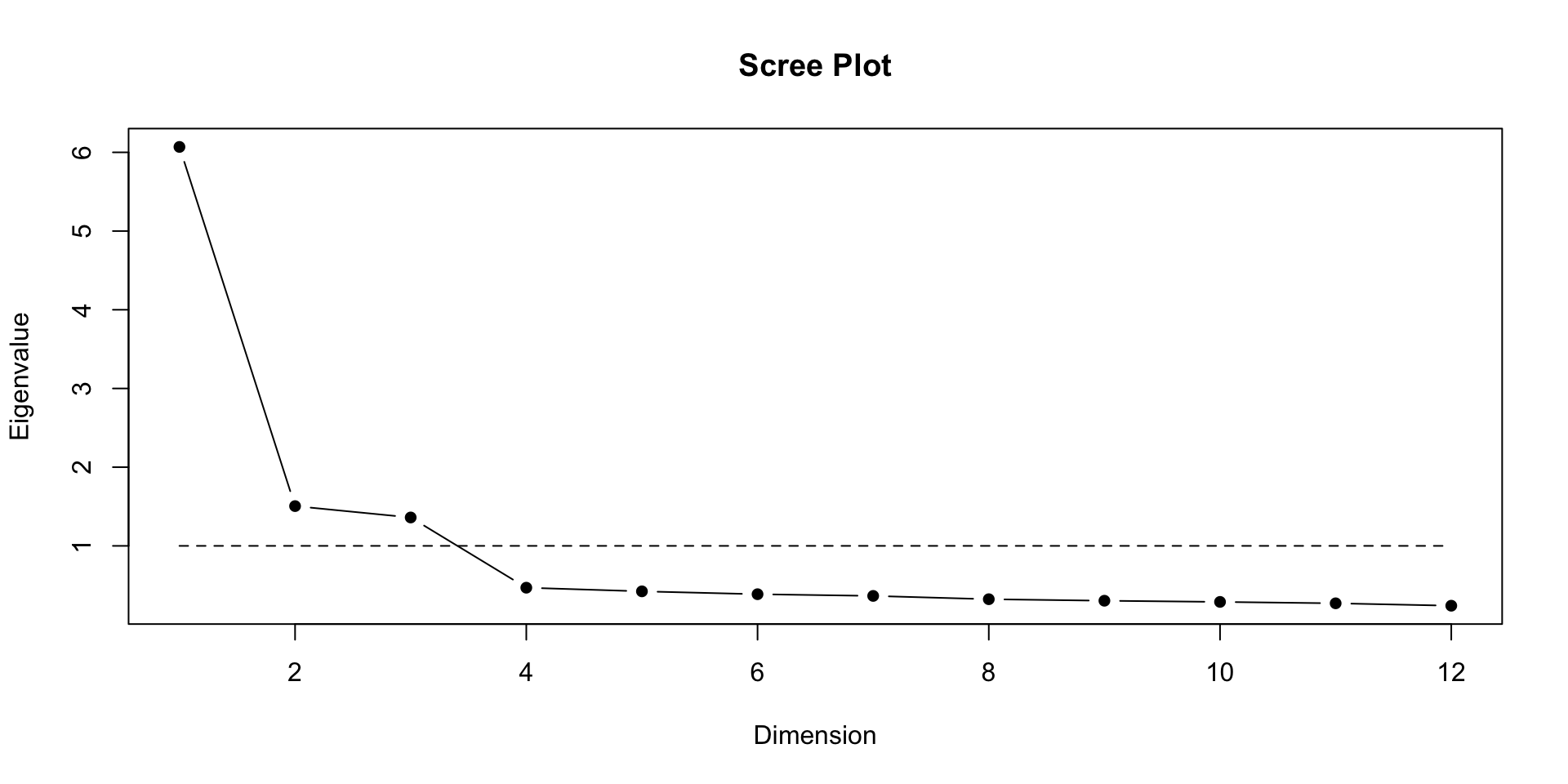
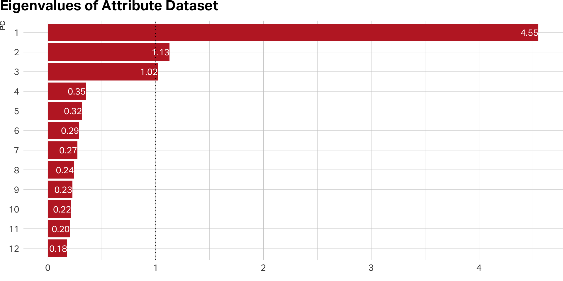
Eigen values
- Each factor has an Eigen Value (EV) that indicates amount of variance it accounts for
- EV for each successive factor has a lower value
- Rule of thumb: EVs over 1 are “stable”
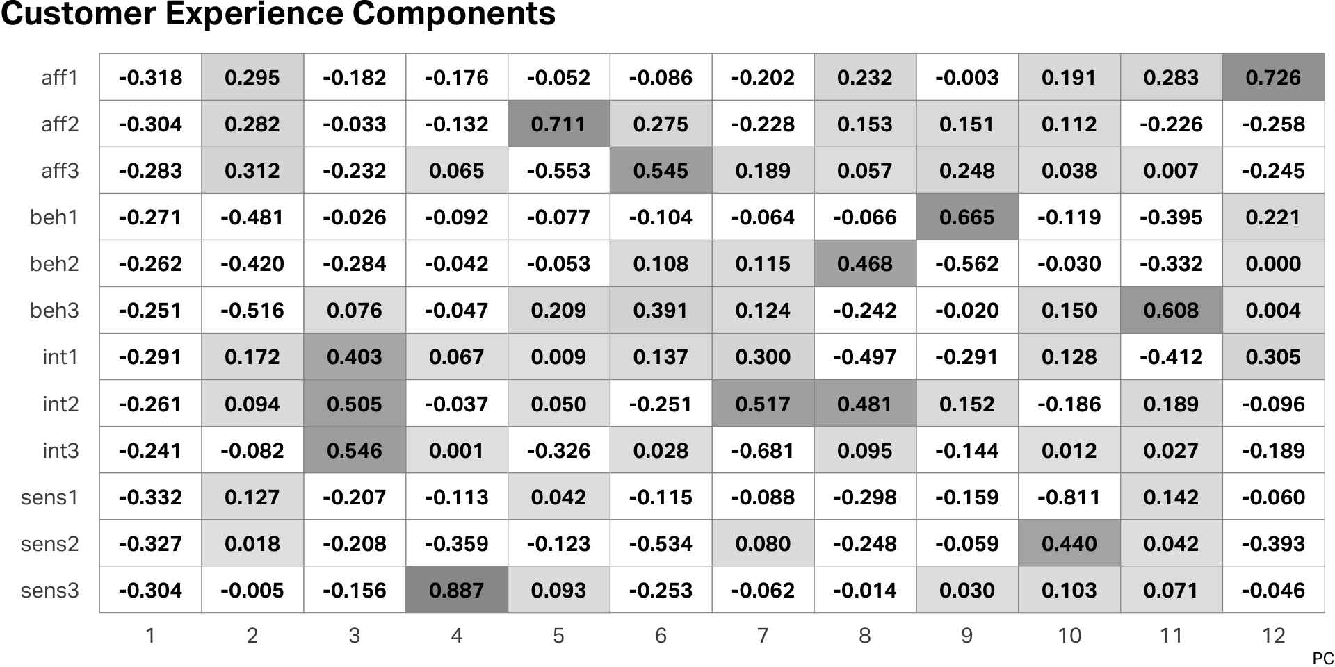
EVs on PCA
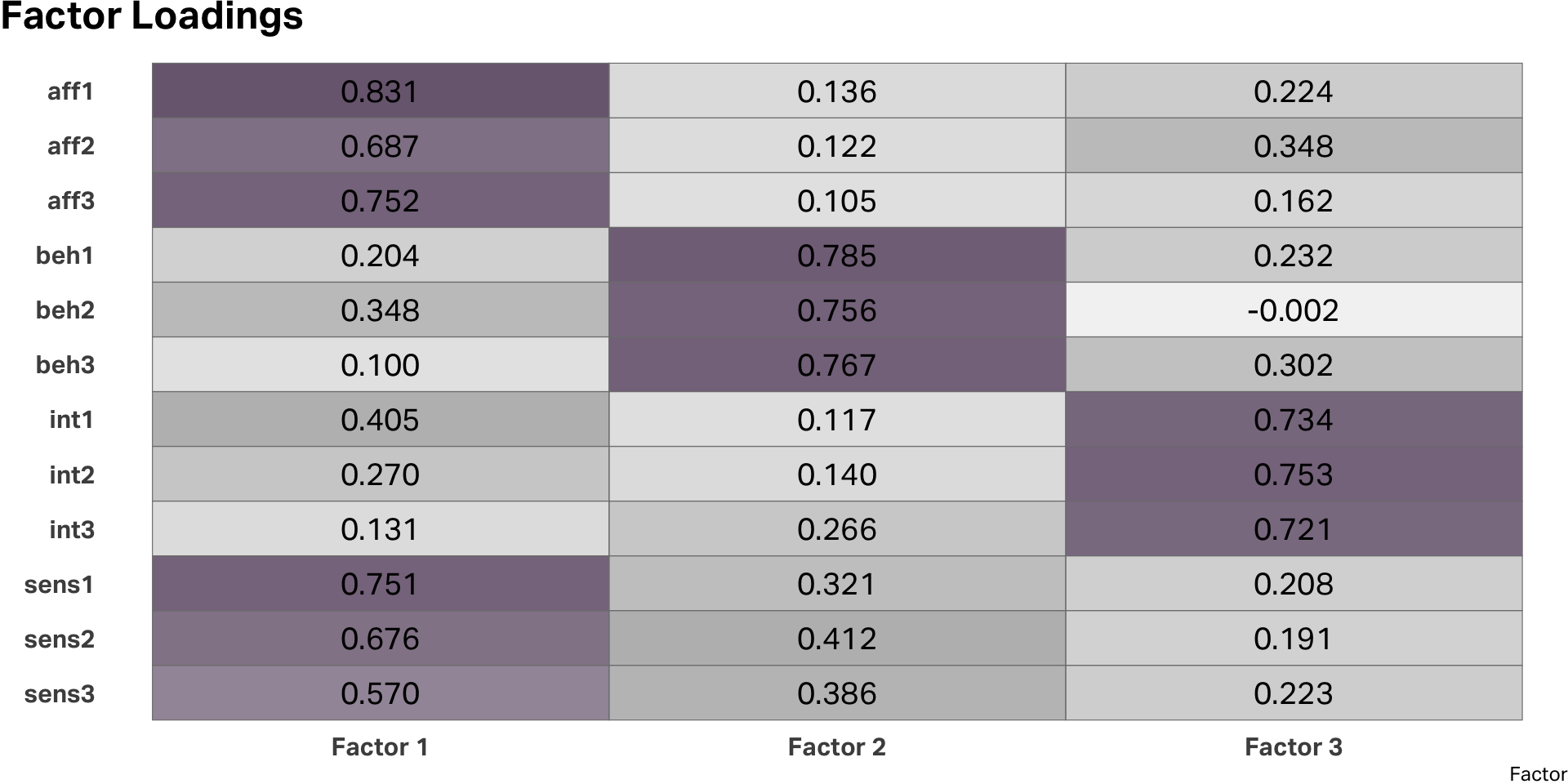
Interpreting the model
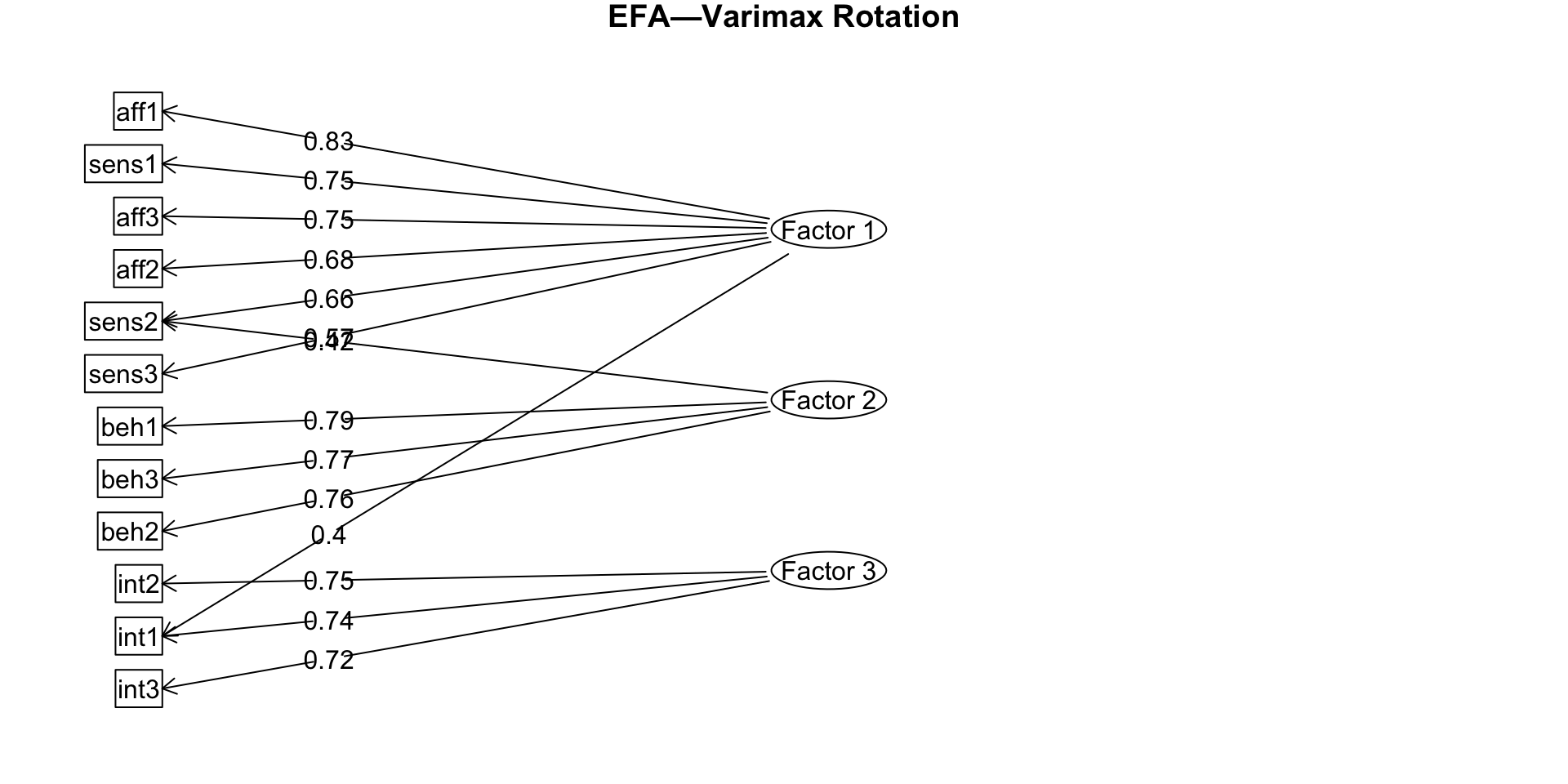
EFA diagram
Uniqueness
| variable | uniqueness |
|---|---|
| sens3 | 0.477 |
| aff3 | 0.397 |
| int3 | 0.392 |
| aff2 | 0.391 |
| int2 | 0.340 |
| sens2 | 0.337 |
| beh3 | 0.310 |
| beh2 | 0.307 |
| sens1 | 0.290 |
| beh1 | 0.288 |
| int1 | 0.283 |
| aff1 | 0.240 |
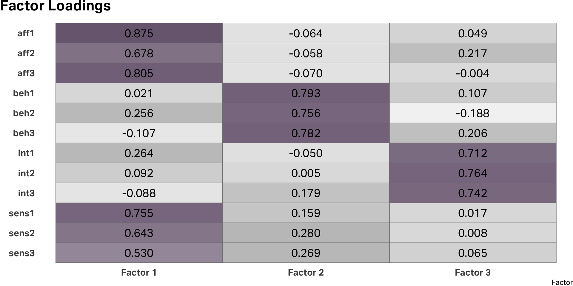
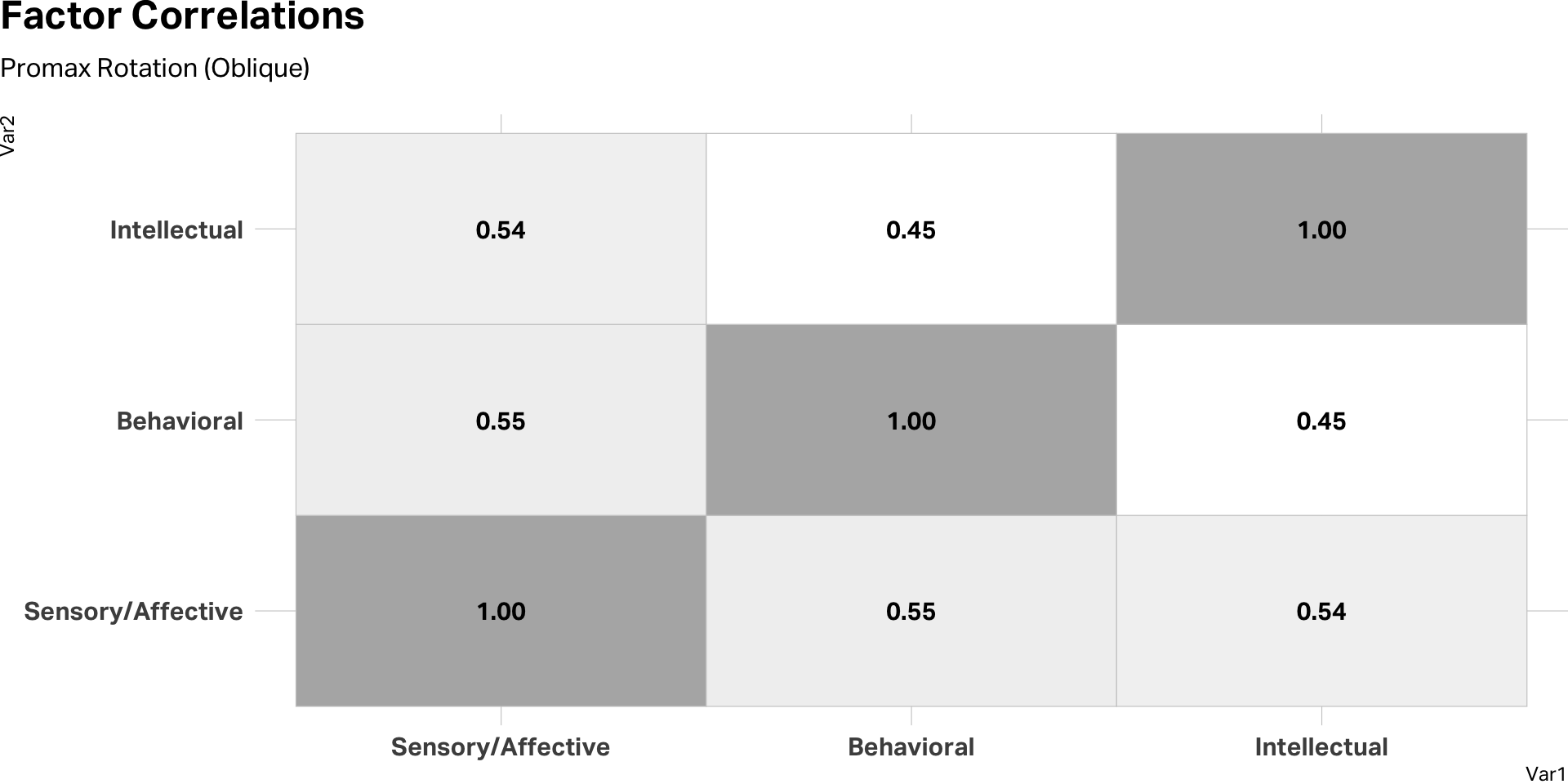
Rotation

Rotated factors
EFA diagram
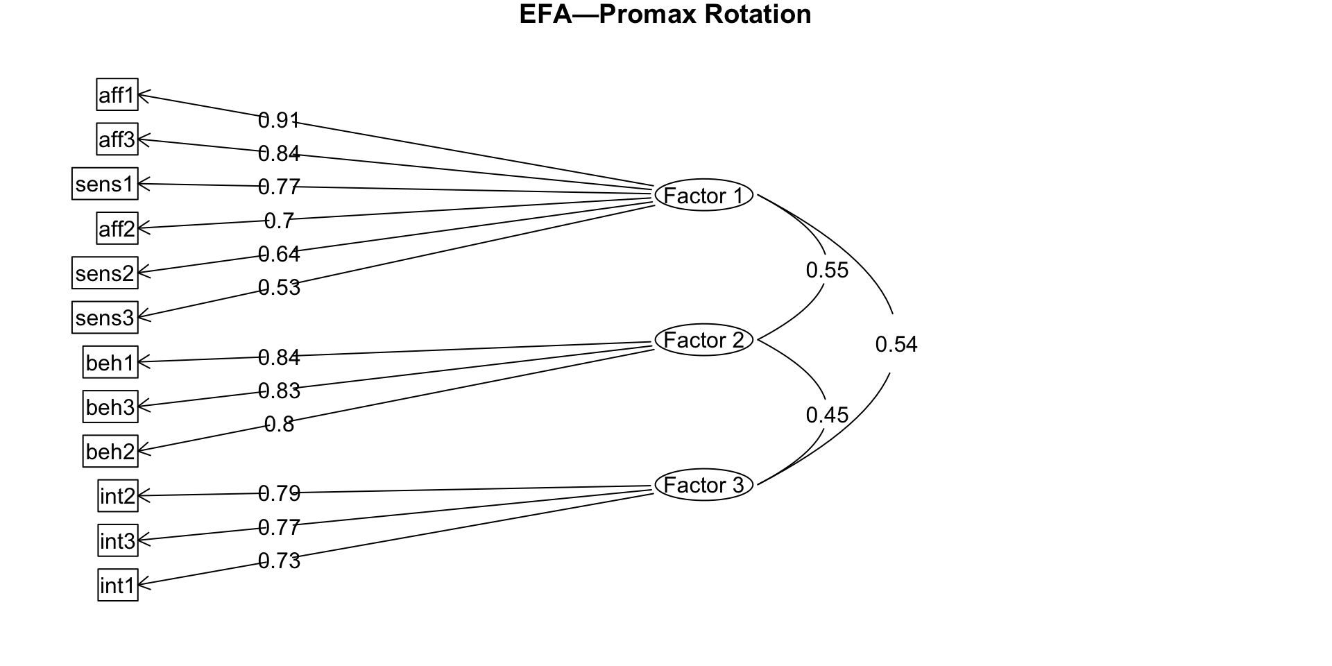
Check correlations
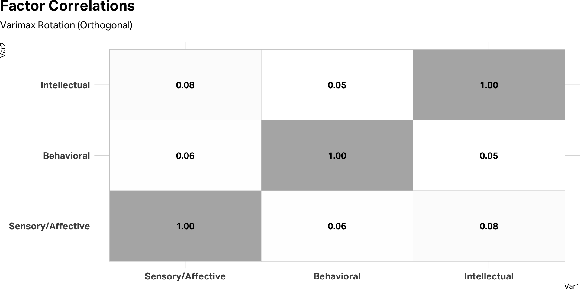
Check correlations
Determine reliability
- Chronbach’s alpha is measure of internal reliability
- Estimates how closely related a set of items are
- Alpha is assessed on a scale from 0-1
Cronbach’s alpha benchmarks
| Alpha | Interpretation |
|---|---|
| α ≥ 0.90 | Excellent |
| 0.80 ≤ α < 0.90 | Good |
| 0.70 ≤ α < 0.80 | Acceptable |
| 0.60 ≤ α < 0.70 | Questionable |
| 0.50 ≤ α < 0.60 | Poor |
| α < 0.50 | Unacceptable |
A note on the ceiling: α above ~0.95 usually indicates item redundancy,
not superior reliability. The sweet spot for a well-constructed scale is 0.80–0.92.
Alpha scores
| Raw Alpha | ||
| factor | raw_alpha | std.alpha |
|---|---|---|
| Sensory/Affective | 0.90 | 0.90 |
| Behavioral | 0.85 | 0.85 |
| Intellectual | 0.84 | 0.84 |
| Alpha Drops | ||
| variable | raw_alpha | std.alpha |
|---|---|---|
| Sensory/Affective | ||
| sens1 | 0.88 | 0.88 |
| sens2 | 0.89 | 0.89 |
| sens3 | 0.90 | 0.90 |
| aff1 | 0.88 | 0.88 |
| aff2 | 0.89 | 0.89 |
| aff3 | 0.89 | 0.89 |
| Behavioral | ||
| beh1 | 0.77 | 0.77 |
| beh2 | 0.82 | 0.82 |
| beh3 | 0.79 | 0.79 |
| Intellectual | ||
| int1 | 0.77 | 0.77 |
| int2 | 0.76 | 0.76 |
| int3 | 0.81 | 0.81 |
Takeaways
What factor analysis offers
Dimension reduction
Many items collapse into a few interpretable scores
Scale validation
Tests whether a theorized construct survives contact with data
Pattern discovery
Surfaces shared variance invisible at the item level
Measurement infrastructure
Composite scores with known reliability feed downstream models
Where to stay skeptical
Statistical structure ≠ latent variable
Items can cluster from wording, response style, or a shared stem
Naming is a theoretical act
A label doesn’t confer ontological status; the math only shows which items covary
Rotation is a claim
Orthogonal vs. oblique is an assertion about the world, not a statistical fact
Replicate before you trust
One sample’s structure isn’t evidence of a general truth
