| estimate | estimate1 | estimate2 | statistic | p.value | conf.low | conf.high |
|---|---|---|---|---|---|---|
| −5.88 | 110.79 | 116.67 | −1.21 | 0.23 | −15.39 | 3.63 |
Analyzing Experimental Data
Overview
Leveraging linear regression to solve a critical customer marketing challenge.
Presented by:
Larry Vincent,
Professor of the Practice
Marketing
Larry Vincent,
Professor of the Practice
Marketing
Presented to:
MKT 512
April 14, 2026
MKT 512
April 14, 2026

Breakout
![]()
- Breakout into smaller groups
- Download the data set (aspen.csv)
- In your group, analyze the data and determine if app users generated more profit in 2020
- The variable
appis the experimental treatment: a 1 means the customer used the app and a 0 means they did not
Difference in groups
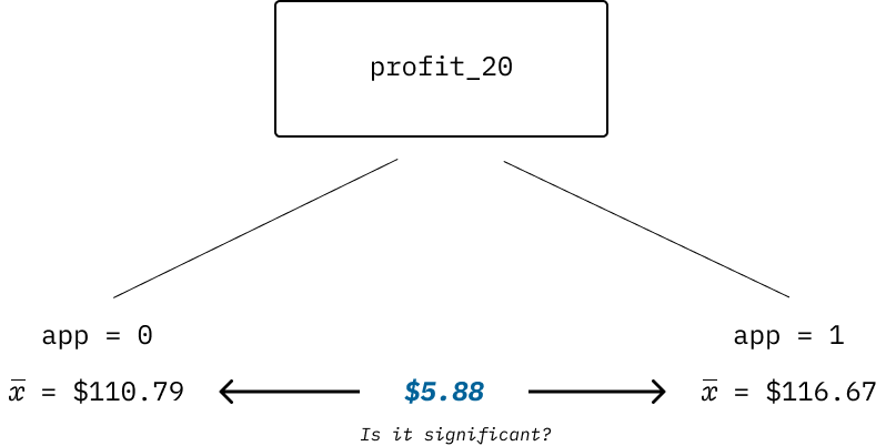
Difference in groups
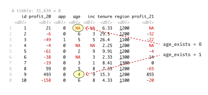
Data inspection
| Statistic | N | Mean | SD | Min | Max | NA |
|---|---|---|---|---|---|---|
| age | 31,634 | 4.05 | 1.64 | 1.00 | 7.00 | 8,289 |
| app | 31,634 | 0.12 | 0.33 | 0.00 | 1.00 | 0 |
| id | 31,634 | 15,817.50 | 9,132.09 | 1.00 | 31,634.00 | 0 |
| inc | 31,634 | 5.46 | 2.35 | 1.00 | 9.00 | 8,261 |
| profit_20 | 31,634 | 111.50 | 272.84 | -221.00 | 2,071.00 | 0 |
| profit_21 | 31,634 | 144.83 | 389.99 | -5,643.00 | 27,086.00 | 5,238 |
| region | 31,634 | 1,203.19 | 47.91 | 1,100.00 | 1,300.00 | 0 |
| tenure | 31,634 | 10.16 | 8.45 | 0.16 | 41.16 | 0 |
Data model
| Dependent variable: | |
| profit_20 | |
| App Only | |
| app | 5.88 (4.69) |
| Constant | 110.79*** (1.64) |
| Observations | 31,634 |
| R2 | 0.0000 |
| Adjusted R2 | 0.0000 |
| Residual Std. Error | 272.84 (df = 31632) |
| F Statistic | 1.57 (df = 1; 31632) |
| Note: | Significance: * p < 0.1, ** p < 0.05, *** p < 0.01 |
Adding in age
| Dependent variable: | ||
| profit_20 | ||
| App Only | App + Age | |
| (1) | (2) | |
| app | 5.88 (4.69) | 27.19*** (5.52) |
| age | 25.86*** (1.12) | |
| Constant | 110.79*** (1.64) | 17.08*** (5.06) |
| Observations | 31,634 | 23,345 |
| R2 | 0.0000 | 0.02 |
| Adjusted R2 | 0.0000 | 0.02 |
| Residual Std. Error | 272.84 (df = 31632) | 278.29 (df = 23342) |
| F Statistic | 1.57 (df = 1; 31632) | 264.95*** (df = 2; 23342) |
| Note: | Significance: * p < 0.1, ** p < 0.05, *** p < 0.01 | |
Breakout
![]()
- Should we or shouldn’t we use the cases with missing data?
- What is the risk of omitting these cases?
Let’s test the influence
Create a new dummy variable age_exists that serves as a predictor. If it has a statistically significant impact on the results, we should be cautious about dropping missing values.
Influence of age
| Dependent variable: | ||
| profit_20 | ||
| App Only | App + Age Exists | |
| (1) | (2) | |
| app | 5.88 (4.69) | 3.56 (4.68) |
| age_exists | 52.14*** (3.48) | |
| Constant | 110.79*** (1.64) | 72.59*** (3.03) |
| Observations | 31,634 | 31,634 |
| R2 | 0.0000 | 0.01 |
| Adjusted R2 | 0.0000 | 0.01 |
| Residual Std. Error | 272.84 (df = 31632) | 271.88 (df = 31631) |
| F Statistic | 1.57 (df = 1; 31632) | 113.14*** (df = 2; 31631) |
| Note: | Significance: * p < 0.1, ** p < 0.05, *** p < 0.01 | |
Average or zero?
| Dependent variable: | ||
| profit_20 | ||
| Age Zero | Age Avg. | |
| (1) | (2) | |
| app | 19.65*** (4.69) | 19.65*** (4.69) |
| age_exists | -51.85*** (5.60) | 51.74*** (3.45) |
| age_zero | 25.60*** (1.09) | |
| age_avg | 25.60*** (1.09) | |
| Constant | 70.93*** (3.00) | -32.66*** (5.38) |
| Observations | 31,634 | 31,634 |
| R2 | 0.02 | 0.02 |
| Adjusted R2 | 0.02 | 0.02 |
| Residual Std. Error (df = 31630) | 269.52 | 269.52 |
| F Statistic (df = 3; 31630) | 262.12*** | 262.12*** |
| Note: | Significance: * p < 0.1, ** p < 0.05, *** p < 0.01 | |
What if we imputed the missing values?
Random forest
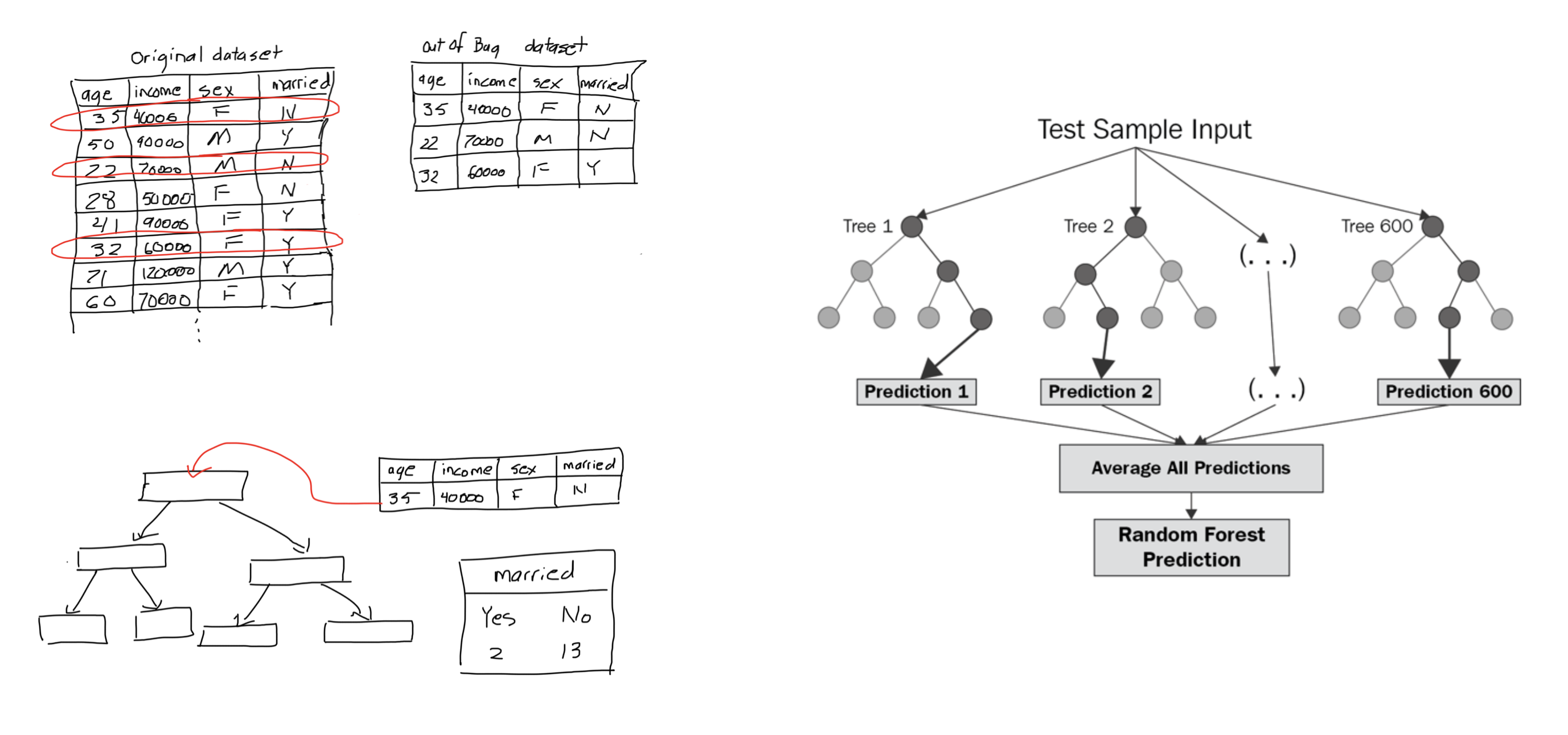
Using random forest
| Dependent variable: | |||
| profit_20 | |||
| Age Zero | Age Avg | Age RF | |
| (1) | (2) | (3) | |
| app | 19.65*** (4.69) | 19.65*** (4.69) | 27.28*** (4.69) |
| age_exists | -51.85*** (5.60) | 51.74*** (3.45) | 47.58*** (3.44) |
| age_zero | 25.60*** (1.09) | ||
| age_avg | 25.60*** (1.09) | ||
| age_rf | 30.52*** (1.07) | ||
| Constant | 70.93*** (3.00) | -32.66*** (5.38) | -49.38*** (5.22) |
| Observations | 31,634 | 31,634 | 31,634 |
| R2 | 0.02 | 0.02 | 0.03 |
| Adjusted R2 | 0.02 | 0.02 | 0.03 |
| Residual Std. Error (df = 31630) | 269.52 | 269.52 | 268.46 |
| F Statistic (df = 3; 31630) | 262.12*** | 262.12*** | 347.45*** |
| Note: | Significance: * p < 0.1, ** p < 0.05, *** p < 0.01 | ||
Adding income
| Dependent variable: | ||
| profit_20 | ||
| App Only | App + Inc | |
| (1) | (2) | |
| app | 5.88 (4.69) | 16.12*** (4.64) |
| age_exists | 9.63 (8.20) | |
| age_rf | 31.81*** (1.06) | |
| inc_exists | 35.24*** (8.21) | |
| inc_rf | 21.89*** (0.74) | |
| Constant | 110.79*** (1.64) | -169.72*** (6.54) |
| Observations | 31,634 | 31,634 |
| R2 | 0.0000 | 0.06 |
| Adjusted R2 | 0.0000 | 0.06 |
| Residual Std. Error | 272.84 (df = 31632) | 264.76 (df = 31628) |
| F Statistic | 1.57 (df = 1; 31632) | 392.78*** (df = 5; 31628) |
| Note: | Significance: * p < 0.1, ** p < 0.05, *** p < 0.01 | |
How should we handle region data?
Adding region
| Dependent variable: | ||
| profit_20 | ||
| App Only | App + Region | |
| (1) | (2) | |
| app | 5.88 (4.69) | 15.73*** (4.64) |
| age_exists | 9.31 (8.20) | |
| age_rf | 32.00*** (1.06) | |
| inc_exists | 35.40*** (8.21) | |
| inc_rf | 21.38*** (0.76) | |
| region1200 | 13.98*** (5.14) | |
| region1300 | 5.96 (6.28) | |
| Constant | 110.79*** (1.64) | -179.07*** (7.71) |
| Observations | 31,634 | 31,634 |
| R2 | 0.0000 | 0.06 |
| Adjusted R2 | 0.0000 | 0.06 |
| Residual Std. Error | 272.84 (df = 31632) | 264.73 (df = 31626) |
| F Statistic | 1.57 (df = 1; 31632) | 281.95*** (df = 7; 31626) |
| Note: | Significance: * p < 0.1, ** p < 0.05, *** p < 0.01 | |
Final model
| Dependent variable: | ||
| profit_20 | ||
| App Only | App + All | |
| (1) | (2) | |
| app | 5.88 (4.69) | 15.88*** (4.61) |
| age_exists | 2.26 (8.15) | |
| age_rf | 21.60*** (1.17) | |
| inc_exists | 32.30*** (8.16) | |
| inc_rf | 19.96*** (0.75) | |
| region1200 | 15.36*** (5.10) | |
| region1300 | 6.04 (6.24) | |
| tenure | 4.08*** (0.20) | |
| Constant | 110.79*** (1.64) | -164.74*** (7.69) |
| Observations | 31,634 | 31,634 |
| R2 | 0.0000 | 0.07 |
| Adjusted R2 | 0.0000 | 0.07 |
| Residual Std. Error | 272.84 (df = 31632) | 262.96 (df = 31625) |
| F Statistic | 1.57 (df = 1; 31632) | 303.71*** (df = 8; 31625) |
| Note: | Significance: * p < 0.1, ** p < 0.05, *** p < 0.01 | |
What about 2021 profitability?
Back to demographics
| Dependent variable: | |
| profit_21 | |
| demographics | 47.53*** (5.98) |
| Constant | 106.86*** (5.34) |
| Observations | 26,396 |
| R2 | 0.002 |
| Adjusted R2 | 0.002 |
| Residual Std. Error | 389.54 (df = 26394) |
| F Statistic | 63.19*** (df = 1; 26394) |
| Note: | Significance: * p < 0.1, ** p < 0.05, *** p < 0.01 |
A better model
| Dependent variable: | |
| profit_21 | |
| app | 18.77*** (5.84) |
| region1200 | 15.10** (6.55) |
| region1300 | 11.21 (8.15) |
| tenure | 0.92*** (0.23) |
| profit_20 | 0.83*** (0.01) |
| Constant | 19.82*** (6.70) |
| Observations | 26,396 |
| R2 | 0.36 |
| Adjusted R2 | 0.36 |
| Residual Std. Error | 312.04 (df = 26390) |
| F Statistic | 2,968.07*** (df = 5; 26390) |
| Note: | Significance: * p < 0.1, ** p < 0.05, *** p < 0.01 |
Region removed
| term | estimate | std.error | statistic | p.value | sig |
|---|---|---|---|---|---|
| (Intercept) | 32.96 | 3.23 | 10.20 | 0.00 | * |
| app | 19.44 | 5.83 | 3.33 | 0.00 | * |
| tenure | 0.90 | 0.23 | 3.94 | 0.00 | * |
| profit_20 | 0.83 | 0.01 | 118.81 | 0.00 | * |
Model Fit
| r.squared | adj.r.squared | sigma | statistic | p.value | df |
|---|---|---|---|---|---|
| 0.36 | 0.36 | 312.06 | 4,944.31 | 0.00 | 3 |
VIF
| variable | value |
|---|---|
| app | 1.01 |
| tenure | 1.04 |
| profit_20 | 1.04 |
What effect does the app have on retention?
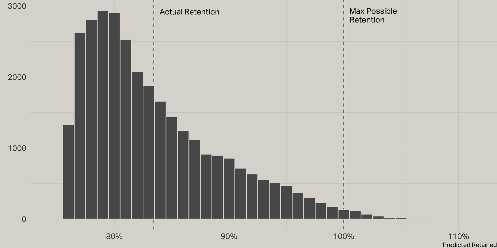
Actual retention

Retention model
| term | estimate | std.error | statistic | p.value | sig |
|---|---|---|---|---|---|
| (Intercept) | 0.76 | 0.00 | 224.82 | 0.00 | * |
| app | 0.03 | 0.01 | 5.10 | 0.00 | * |
| tenure | 0.01 | 0.00 | 25.57 | 0.00 | * |
| profit_20 | 0.00 | 0.00 | 7.17 | 0.00 | * |
Model Fit
| r.squared | adj.r.squared | sigma | statistic | p.value | df |
|---|---|---|---|---|---|
| 0.03 | 0.03 | 0.37 | 272.26 | 0.00 | 3 |
Predictions
Logistic regression
Logistic regression model
| term | estimate | std.error | statistic | p.value | sig |
|---|---|---|---|---|---|
| (Intercept) | 1.03 | 0.02 | 42.71 | 0.00 | * |
| app | 0.23 | 0.05 | 4.81 | 0.00 | * |
| profit_20 | 0.00 | 0.00 | 7.38 | 0.00 | * |
| tenure | 0.06 | 0.00 | 24.78 | 0.00 | * |
Logistic function
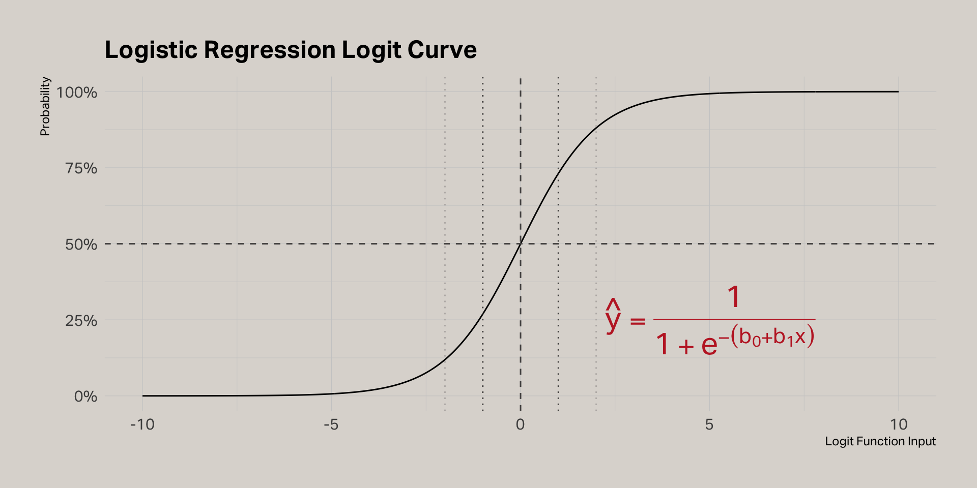
Translating log-odds to probabilities
| term | estimate | std.error | statistic | p.value | odds | p | sig |
|---|---|---|---|---|---|---|---|
| (Intercept) | 1.03 | 0.02 | 42.71 | 0.00 | 2.81 | 0.74 | * |
| app | 0.23 | 0.05 | 4.81 | 0.00 | 1.26 | 0.56 | * |
| profit_20 | 0.00 | 0.00 | 7.38 | 0.00 | 1.00 | 0.50 | * |
| tenure | 0.06 | 0.00 | 24.78 | 0.00 | 1.06 | 0.51 | * |
Interpreting
- Like linear regression, add the estimates to the intercept to determine the impact of each coefficient
- The estimates are expressed in log-odds, which is the logarithm of the odds ratio
- The odds ratio is the odds of an outcome happening given a treatment compared to the odds of the outcome happening without the treatment
- An odds ratio of 1 means there is equal chance of the outcome, with or without the treatment
- To calculate the odds ratio, simply take the exponent of the coefficient provided by the model
- To calculate the probability for a coefficient, divide the odds ratio by (1 + odds ratio)
Interpreting our model
| term | estimate | std.error | statistic | p.value | odds | p | sig |
|---|---|---|---|---|---|---|---|
| (Intercept) | 1.03 | 0.02 | 42.71 | 0.00 | 2.81 | 0.74 | * |
| app | 0.23 | 0.05 | 4.81 | 0.00 | 1.26 | 0.56 | * |
| profit_20 | 0.00 | 0.00 | 7.38 | 0.00 | 1.00 | 0.50 | * |
| tenure | 0.06 | 0.00 | 24.78 | 0.00 | 1.06 | 0.51 | * |
- 74% probability of retention if all terms are zero
- On its own, the app increases the probability of retention by 56%
- To calculate the retention probability for a customer using the app, first calculate the odds ratio = exponent(1.03 + 0.23 = 1.26) = 3.52
- Then, you can estimate the probability of retention = 3.52 / (1 + 3.52) = 77%
- This estimate assumes tenure = 0 and 2020 profit = 0 (e.g., a new customer)
Profit 2020
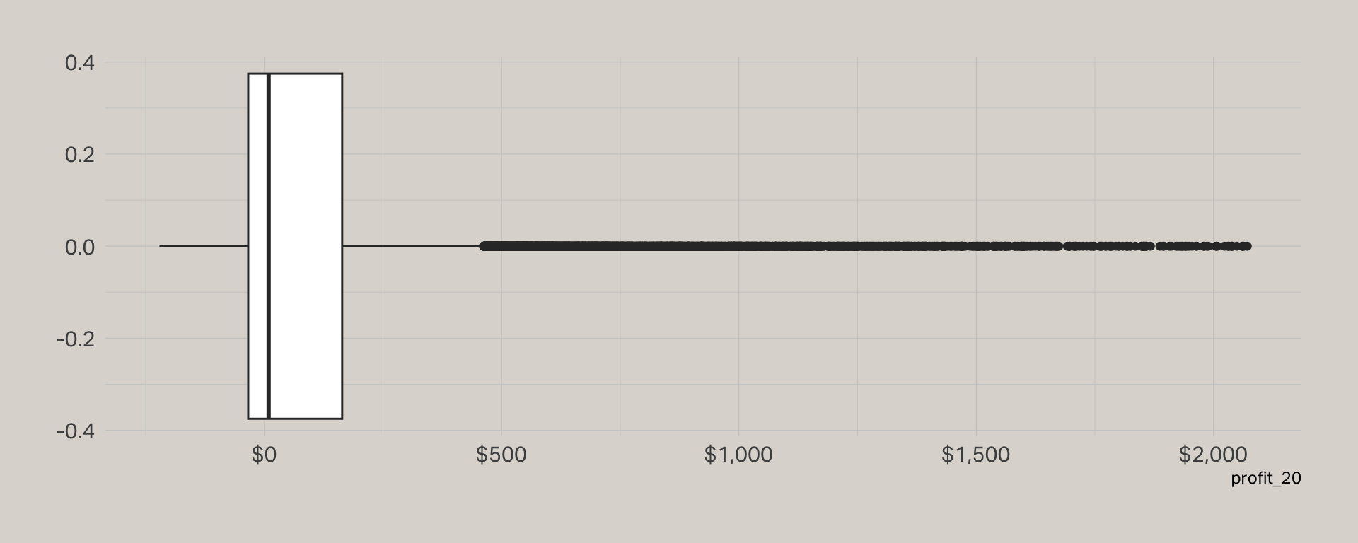
Rescaling
| term | estimate | std.error | statistic | p.value | odds | p | sig |
|---|---|---|---|---|---|---|---|
| (Intercept) | 0.92 | 0.03 | 30.75 | 0.00 | 2.51 | 0.72 | * |
| app | 0.23 | 0.05 | 4.81 | 0.00 | 1.26 | 0.56 | * |
| profit_20 | 1.18 | 0.16 | 7.38 | 0.00 | 3.25 | 0.76 | * |
| tenure | 0.06 | 0.00 | 24.78 | 0.00 | 1.06 | 0.51 | * |
Where is R squared?
Assessing fit

Training model
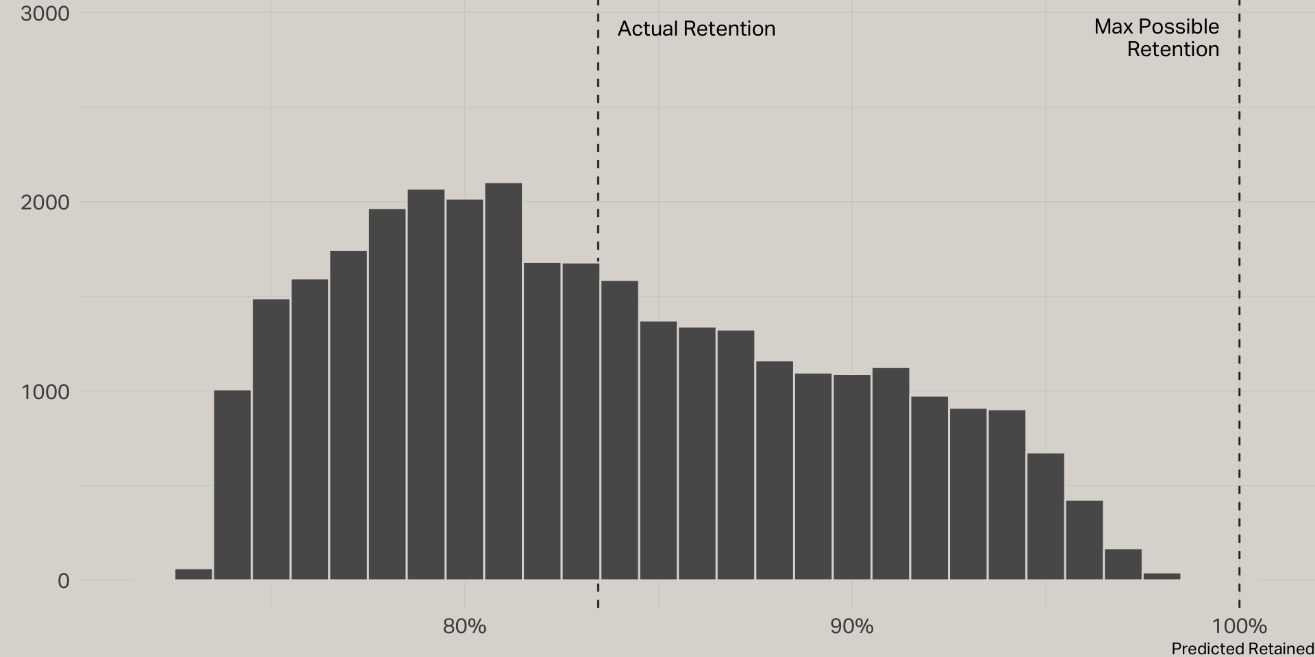
In the initial logistic regression model, 83% of cases actually were retained. This resulted in a lopsided model that predicted all cases in the test set were retained, when in fact 16% were not. To compensate, I trained a new model using a test set that had equal proportions of retained and churned customers. This was accomplished by undersampling retained cases.
| term | estimate | std.error | statistic | p.value | odds | p | sig |
|---|---|---|---|---|---|---|---|
| (Intercept) | 0.08 | 0.02 | 3.40 | 0.00 | 1.08 | 0.52 | * |
| app | 0.07 | 0.02 | 3.21 | 0.00 | 1.08 | 0.52 | * |
| profit_20 | 0.14 | 0.03 | 5.44 | 0.00 | 1.15 | 0.54 | * |
| tenure | 0.46 | 0.03 | 17.20 | 0.00 | 1.58 | 0.61 | * |