| variable | Median | Mean | SD | Min | Max | N | NA |
|---|---|---|---|---|---|---|---|
| engine_size | 4 | 4.06 | 1.53 | 1.00 | 7.00 | 100 | 0 |
| horsepower | 4 | 4.11 | 1.44 | 1.00 | 7.00 | 100 | 0 |
| intent | 5 | 4.48 | 1.45 | 1.00 | 7.00 | 100 | 0 |
| sound_system | 4 | 3.51 | 1.13 | 1.00 | 7.00 | 100 | 0 |
| torque | 4 | 3.75 | 1.39 | 1.00 | 7.00 | 100 | 0 |
Aspen Homegoods (B)
Overview
Using logistic regression approaches to solve a retention question.
Presented by:
Larry Vincent,
Professor of the Practice
Marketing
Larry Vincent,
Professor of the Practice
Marketing
Presented to:
MKT 512
November 6, 2025
MKT 512
November 6, 2025

Multicolinearity effects

Auto Case
- Intent to purchase based on survey data
- Importance attributes: engine_size, horsepower, torque, sound_system
- All responses answered on a
7-point scale
Dataset
Correlations
| column | intent | engine_size | horsepower | torque | sound_system |
|---|---|---|---|---|---|
| intent | 1.00 | 0.68 | 0.68 | 0.69 | 0.52 |
| engine_size | 0.68 | 1.00 | 0.91 | 0.78 | −0.15 |
| horsepower | 0.68 | 0.91 | 1.00 | 0.68 | −0.08 |
| torque | 0.69 | 0.78 | 0.68 | 1.00 | −0.10 |
| sound_system | 0.52 | −0.15 | −0.08 | −0.10 | 1.00 |
Regression
| term | estimate | std.error | statistic | p.value | sig |
|---|---|---|---|---|---|
| (Intercept) | −1.83 | 0.18 | −9.95 | 0.00 | * |
| engine_size | 0.17 | 0.08 | 2.25 | 0.03 | * |
| horsepower | 0.29 | 0.07 | 4.33 | 0.00 | * |
| torque | 0.43 | 0.05 | 9.52 | 0.00 | * |
| sound_system | 0.79 | 0.04 | 22.45 | 0.00 | * |
Model Fit
| r.squared | adj.r.squared | sigma | statistic | p.value | df |
|---|---|---|---|---|---|
| 0.93 | 0.93 | 0.39 | 317.54 | 0.00 | 4 |
Variance inflation factors
Regression
| term | estimate | std.error | statistic | p.value | sig |
|---|---|---|---|---|---|
| (Intercept) | −1.83 | 0.18 | −9.95 | 0.00 | * |
| engine_size | 0.17 | 0.08 | 2.25 | 0.03 | * |
| horsepower | 0.29 | 0.07 | 4.33 | 0.00 | * |
| torque | 0.43 | 0.05 | 9.52 | 0.00 | * |
| sound_system | 0.79 | 0.04 | 22.45 | 0.00 | * |
Model Fit
| r.squared | adj.r.squared | sigma | statistic | p.value | df |
|---|---|---|---|---|---|
| 0.93 | 0.93 | 0.39 | 317.54 | 0.00 | 4 |
VIF
| variable | value |
|---|---|
| engine_size | 8.66 |
| horsepower | 6.22 |
| torque | 2.58 |
| sound_system | 1.04 |
Model with one predictor
| term | estimate | std.error | statistic | p.value |
|---|---|---|---|---|
| (Intercept) | 1.87 | 0.31 | 6.10 | 0.00 |
| engine_size | 0.64 | 0.07 | 9.13 | 0.00 |
Model Fit
| r.squared | adj.r.squared | sigma | statistic | p.value | df |
|---|---|---|---|---|---|
| 0.46 | 0.45 | 1.07 | 83.28 | 0.00 | 1 |
Model with sound predictor
| term | estimate | std.error | statistic | p.value |
|---|---|---|---|---|
| (Intercept) | 2.12 | 0.41 | 5.21 | 0.00 |
| sound_system | 0.67 | 0.11 | 6.11 | 0.00 |
Model Fit
| r.squared | adj.r.squared | sigma | statistic | p.value | df |
|---|---|---|---|---|---|
| 0.28 | 0.27 | 1.24 | 37.29 | 0.00 | 1 |
Combined model
| term | estimate | std.error | statistic | p.value | sig |
|---|---|---|---|---|---|
| (Intercept) | −1.36 | 0.25 | −5.41 | 0.00 | * |
| engine_size | 0.73 | 0.04 | 19.89 | 0.00 | * |
| sound_system | 0.82 | 0.05 | 16.45 | 0.00 | * |
Model Fit
| r.squared | adj.r.squared | sigma | statistic | p.value | df |
|---|---|---|---|---|---|
| 0.86 | 0.85 | 0.55 | 291.39 | 0.00 | 2 |
VIF
| variable | value |
|---|---|
| engine_size | 1.02 |
| sound_system | 1.02 |
Can we go for more?
| term | estimate | std.error | statistic | p.value | sig |
|---|---|---|---|---|---|
| (Intercept) | −1.70 | 0.20 | −8.61 | 0.00 | * |
| engine_size | 0.45 | 0.04 | 9.95 | 0.00 | * |
| torque | 0.41 | 0.05 | 8.27 | 0.00 | * |
| sound_system | 0.81 | 0.04 | 21.29 | 0.00 | * |
Model Fit
| r.squared | adj.r.squared | sigma | statistic | p.value | df |
|---|---|---|---|---|---|
| 0.92 | 0.91 | 0.43 | 352.03 | 0.00 | 3 |
VIF
| variable | value |
|---|---|
| engine_size | 2.56 |
| torque | 2.53 |
| sound_system | 1.02 |
What about horsepower instead?
| term | estimate | std.error | statistic | p.value | sig |
|---|---|---|---|---|---|
| (Intercept) | −1.44 | 0.25 | −5.76 | 0.00 | * |
| engine_size | 0.56 | 0.09 | 6.24 | 0.00 | * |
| horsepower | 0.20 | 0.09 | 2.18 | 0.03 | * |
| sound_system | 0.80 | 0.05 | 16.37 | 0.00 | * |
Model Fit
| r.squared | adj.r.squared | sigma | statistic | p.value | df |
|---|---|---|---|---|---|
| 0.86 | 0.86 | 0.54 | 203.35 | 0.00 | 3 |
VIF
| variable | value |
|---|---|
| engine_size | 6.19 |
| horsepower | 6.10 |
| sound_system | 1.04 |
Back to Aspen
Correlations
| column | profit_20 | app | age | inc | tenure | region |
|---|---|---|---|---|---|---|
| profit_20 | 1.00 | 0.01 | 0.14 | 0.15 | 0.17 | 0.00 |
| app | 0.01 | 1.00 | −0.17 | 0.09 | −0.08 | 0.01 |
| age | 0.14 | −0.17 | 1.00 | −0.08 | 0.42 | −0.03 |
| inc | 0.15 | 0.09 | −0.08 | 1.00 | 0.03 | 0.03 |
| tenure | 0.17 | −0.08 | 0.42 | 0.03 | 1.00 | −0.01 |
| region | 0.00 | 0.01 | −0.03 | 0.03 | −0.01 | 1.00 |
Final model
| term | estimate | std.error | statistic | p.value | sig |
|---|---|---|---|---|---|
| (Intercept) | 19.82 | 6.70 | 2.96 | 0.00 | * |
| app | 18.77 | 5.84 | 3.21 | 0.00 | * |
| region_1200 | 15.10 | 6.55 | 2.30 | 0.02 | * |
| region_1300 | 11.21 | 8.15 | 1.37 | 0.17 | |
| tenure | 0.92 | 0.23 | 4.02 | 0.00 | * |
| profit_20 | 0.83 | 0.01 | 118.55 | 0.00 | * |
Model Fit
| r.squared | adj.r.squared | sigma | statistic | p.value | df |
|---|---|---|---|---|---|
| 0.36 | 0.36 | 312.04 | 2,968.07 | 0.00 | 5 |
VIF
| variable | value |
|---|---|
| app | 1.01 |
| region_1200 | 2.04 |
| region_1300 | 2.03 |
| tenure | 1.04 |
| profit_20 | 1.04 |
Region removed
| term | estimate | std.error | statistic | p.value | sig |
|---|---|---|---|---|---|
| (Intercept) | 32.96 | 3.23 | 10.20 | 0.00 | * |
| app | 19.44 | 5.83 | 3.33 | 0.00 | * |
| tenure | 0.90 | 0.23 | 3.94 | 0.00 | * |
| profit_20 | 0.83 | 0.01 | 118.81 | 0.00 | * |
Model Fit
| r.squared | adj.r.squared | sigma | statistic | p.value | df |
|---|---|---|---|---|---|
| 0.36 | 0.36 | 312.06 | 4,944.31 | 0.00 | 3 |
VIF
| variable | value |
|---|---|
| app | 1.01 |
| tenure | 1.04 |
| profit_20 | 1.04 |
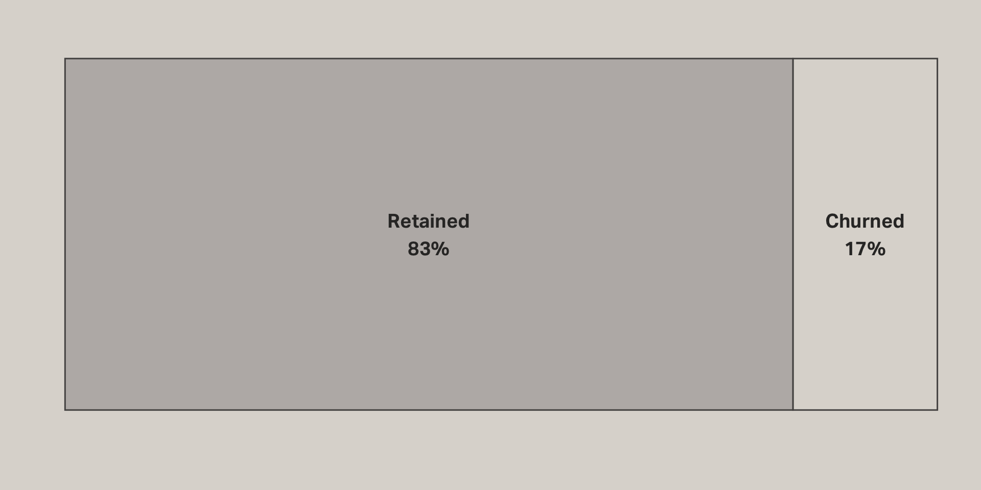
What effect does the app have on retention?
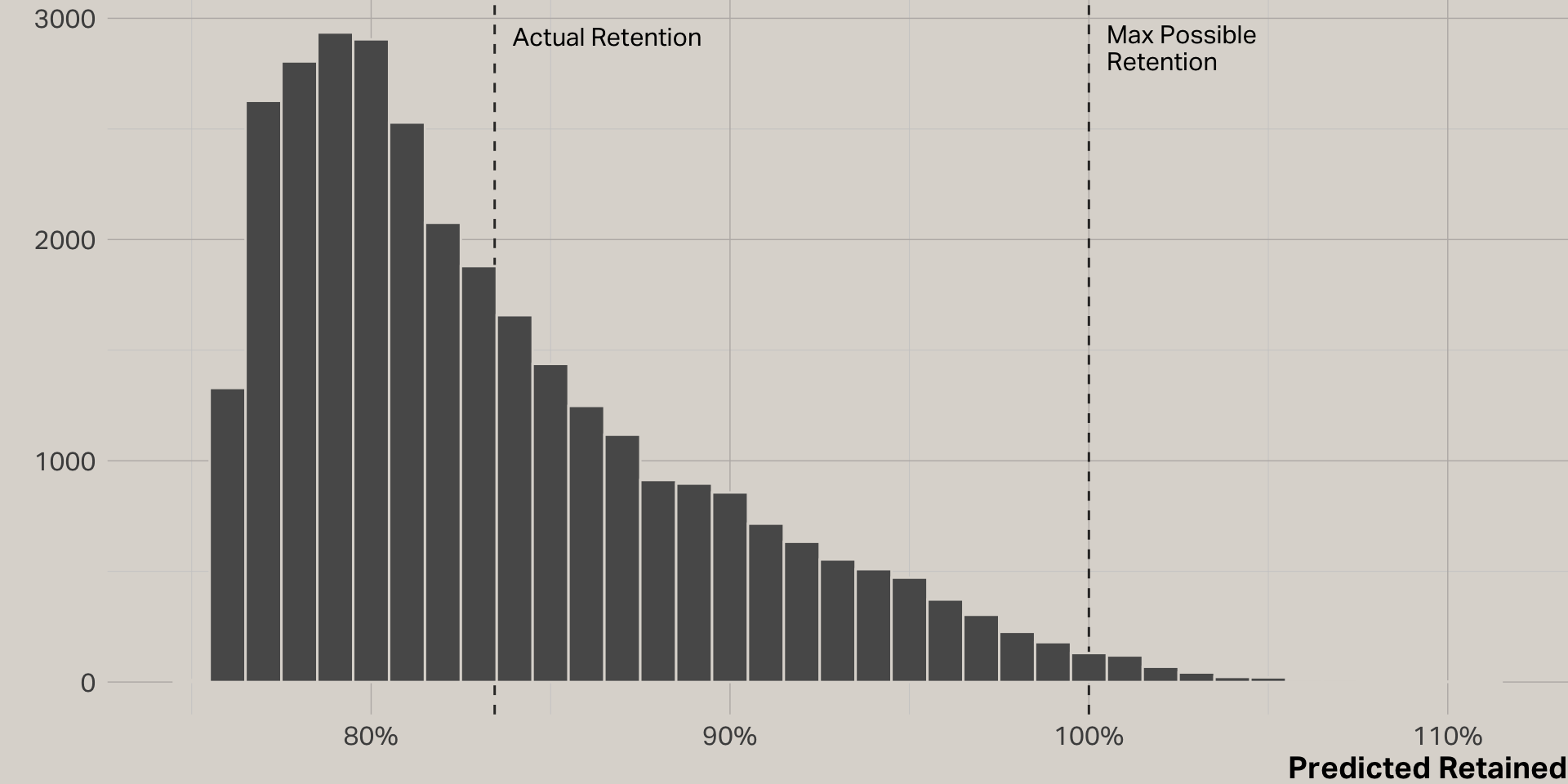
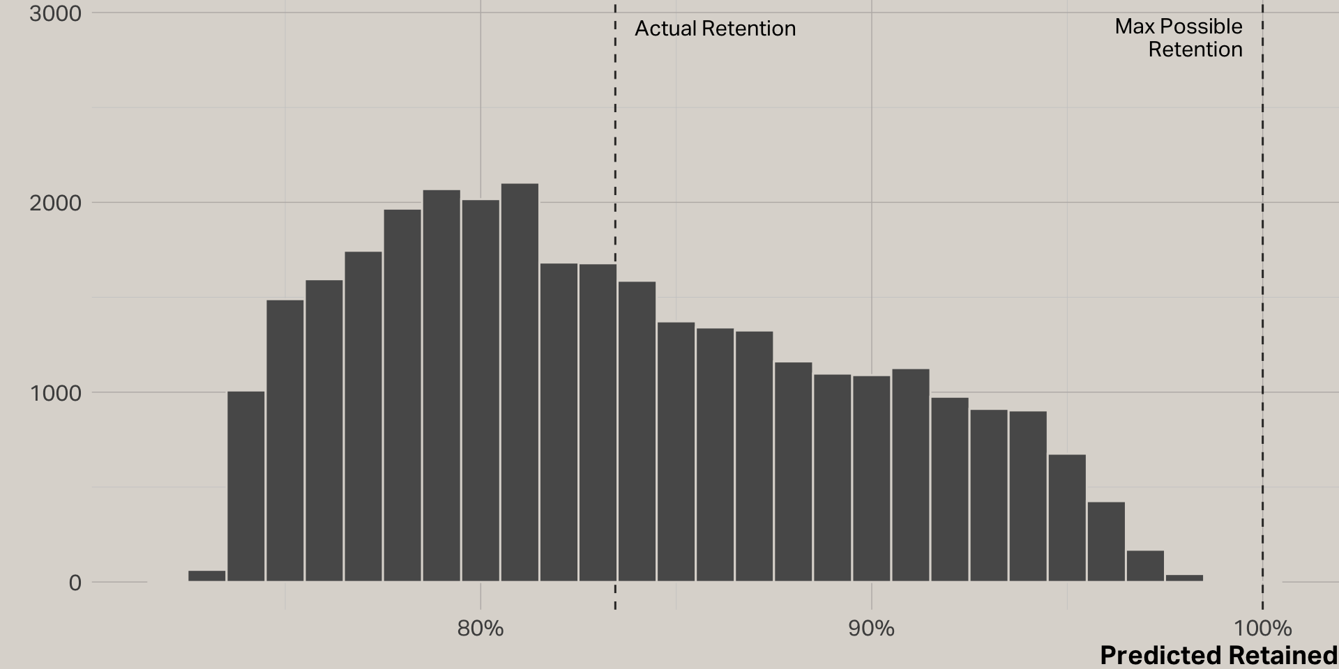
Actual retention
Retention model
| term | estimate | std.error | statistic | p.value | sig |
|---|---|---|---|---|---|
| (Intercept) | 0.76 | 0.00 | 224.82 | 0.00 | * |
| app | 0.03 | 0.01 | 5.10 | 0.00 | * |
| tenure | 0.01 | 0.00 | 25.57 | 0.00 | * |
| profit_20 | 0.00 | 0.00 | 7.17 | 0.00 | * |
Model Fit
| r.squared | adj.r.squared | sigma | statistic | p.value | df |
|---|---|---|---|---|---|
| 0.03 | 0.03 | 0.37 | 272.26 | 0.00 | 3 |
Predictions
Logistic regression
Logistic regression model
| term | estimate | std.error | statistic | p.value | sig |
|---|---|---|---|---|---|
| (Intercept) | 1.03 | 0.02 | 42.71 | 0.00 | * |
| app | 0.23 | 0.05 | 4.81 | 0.00 | * |
| profit_20 | 0.00 | 0.00 | 7.38 | 0.00 | * |
| tenure | 0.06 | 0.00 | 24.78 | 0.00 | * |
Logistic function
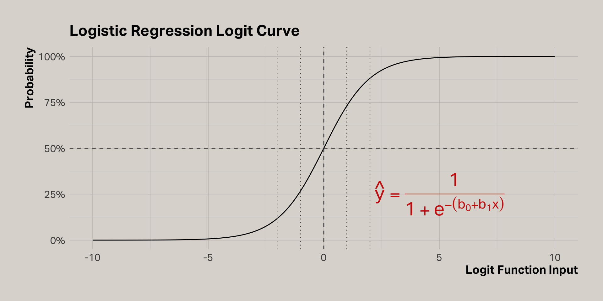
Translating log-odds to probabilities
| term | estimate | std.error | statistic | p.value | odds | p | sig |
|---|---|---|---|---|---|---|---|
| (Intercept) | 1.03 | 0.02 | 42.71 | 0.00 | 2.81 | 0.74 | * |
| app | 0.23 | 0.05 | 4.81 | 0.00 | 1.26 | 0.56 | * |
| profit_20 | 0.00 | 0.00 | 7.38 | 0.00 | 1.00 | 0.50 | * |
| tenure | 0.06 | 0.00 | 24.78 | 0.00 | 1.06 | 0.51 | * |
Interpreting
- Like linear regression, add the estimates to the intercept to determine the impact of each coefficient
- The estimates are expressed in log-odds, which is the logarithm of the odds ratio
- The odds ratio is the odds of an outcome happening given a treatment compared to the odds of the outcome happening without the treatment
- An odds ratio of 1 means there is equal chance of the outcome, with or without the treatment
- To calculate the odds ratio, simply take the exponent of the coefficient provided by the model
- To calculate the probability for a coefficient, divide the odds ratio by (1 + odds ratio)
Interpreting our model
| term | estimate | std.error | statistic | p.value | odds | p | sig |
|---|---|---|---|---|---|---|---|
| (Intercept) | 1.03 | 0.02 | 42.71 | 0.00 | 2.81 | 0.74 | * |
| app | 0.23 | 0.05 | 4.81 | 0.00 | 1.26 | 0.56 | * |
| profit_20 | 0.00 | 0.00 | 7.38 | 0.00 | 1.00 | 0.50 | * |
| tenure | 0.06 | 0.00 | 24.78 | 0.00 | 1.06 | 0.51 | * |
- 74% probability of retention if all terms are zero
- On its own, the app increases the probability of retention by 56%
- To calculate the retention probability for a customer using the app, first calculate the odds ratio = exponent(1.03 + 0.23 = 1.26) = 3.52
- Then, you can estimate the probability of retention = 3.52 / (1 + 3.52) = 77%
- This estimate assumes tenure = 0 and 2020 profit = 0 (e.g., a new customer)
Profit 2020
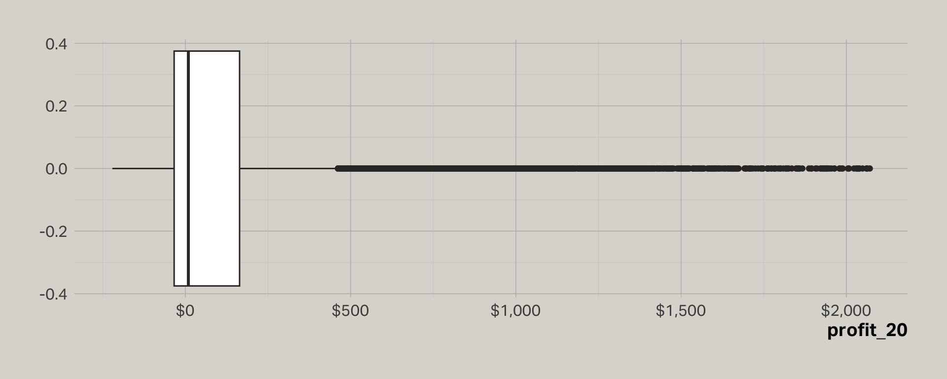
Rescaling
| term | estimate | std.error | statistic | p.value | odds | p | sig |
|---|---|---|---|---|---|---|---|
| (Intercept) | 0.92 | 0.03 | 30.75 | 0.00 | 2.51 | 0.72 | * |
| app | 0.23 | 0.05 | 4.81 | 0.00 | 1.26 | 0.56 | * |
| profit_20 | 1.18 | 0.16 | 7.38 | 0.00 | 3.25 | 0.76 | * |
| tenure | 0.06 | 0.00 | 24.78 | 0.00 | 1.06 | 0.51 | * |
Where is R squared?
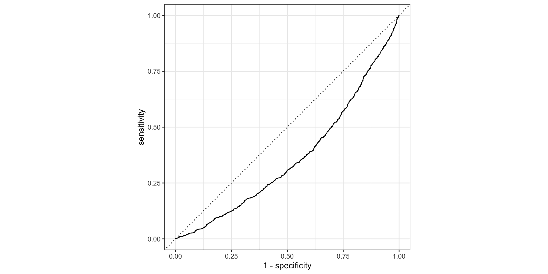
Assessing fit
Training model
In the initial logistic regression model, 83% of cases actually were retained. This resulted in a lopsided model that predicted all cases in the test set were retained, when in fact 16% were not. To compensate, I trained a new model using a test set that had equal proportions of retained and churned customers. This was accomplished by undersampling retained cases.
| term | estimate | std.error | statistic | p.value | odds | p | sig |
|---|---|---|---|---|---|---|---|
| (Intercept) | 0.08 | 0.02 | 3.40 | 0.00 | 1.08 | 0.52 | * |
| app | 0.07 | 0.02 | 3.21 | 0.00 | 1.08 | 0.52 | * |
| profit_20 | 0.14 | 0.03 | 5.44 | 0.00 | 1.15 | 0.54 | * |
| tenure | 0.46 | 0.03 | 17.20 | 0.00 | 1.58 | 0.61 | * |
Accuracy
Confusion matrix
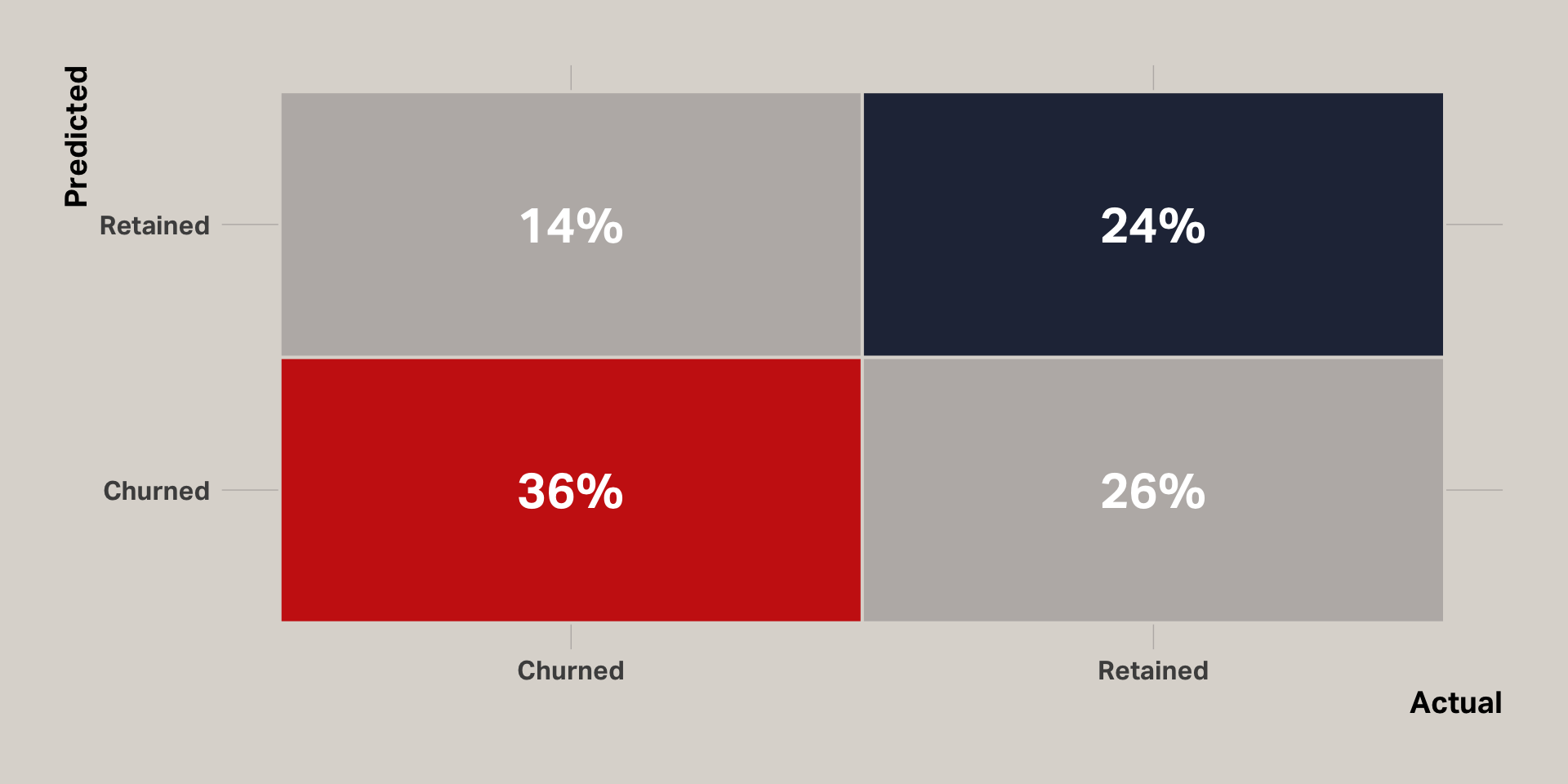
Our model is about 10% better than flipping a coin
Takeaways
- Multicolinearity is an issue to consider when you have high correlations among predictor variables. VIF can be used to assess the inflation effect of correlated predictors.
- Logistic regression is usually the best option when the dependent variable is binary. However, it can be harder to interpret and assess fit.
- Overall, our model demonstrated that the app does have an effect on retention. On its own, the app increases the probability of retention by 52%. And the model predicted the outcome 60% of the time.
