| Statistic | N | Mean | SD | Min | Max | NA |
|---|---|---|---|---|---|---|
| age | 31,634 | 4.05 | 1.64 | 1.00 | 7.00 | 8,289 |
| app | 31,634 | 0.12 | 0.33 | 0.00 | 1.00 | 0 |
| id | 31,634 | 15,817.50 | 9,132.09 | 1.00 | 31,634.00 | 0 |
| inc | 31,634 | 5.46 | 2.35 | 1.00 | 9.00 | 8,261 |
| profit_20 | 31,634 | 111.50 | 272.84 | -221.00 | 2,071.00 | 0 |
| profit_21 | 31,634 | 144.83 | 389.99 | -5,643.00 | 27,086.00 | 5,238 |
| region | 31,634 | 1,203.19 | 47.91 | 1,100.00 | 1,300.00 | 0 |
| tenure | 31,634 | 10.16 | 8.45 | 0.16 | 41.16 | 0 |
Aspen Homegoods (A)
Overview
Leveraging linear regression to solve a critical customer marketing challenge.
Presented by:
Larry Vincent,
Professor of the Practice
Marketing
Larry Vincent,
Professor of the Practice
Marketing
Presented to:
MKT 512
November 4, 2025
MKT 512
November 4, 2025

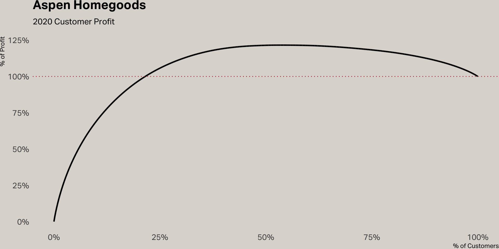
Data inspection
Customer profitability
Difference in groups
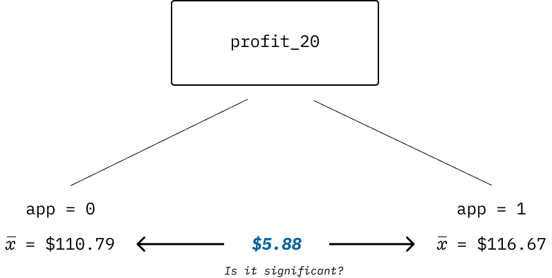
Difference in groups
| estimate | estimate1 | estimate2 | statistic | p.value | conf.low | conf.high |
|---|---|---|---|---|---|---|
| −5.88 | 110.79 | 116.67 | −1.21 | 0.23 | −15.39 | 3.63 |
Data model
| Dependent variable: | |
| profit_20 | |
| app | 5.88 (4.69) |
| Constant | 110.79*** (1.64) |
| Observations | 31,634 |
| R2 | 0.0000 |
| Adjusted R2 | 0.0000 |
| Residual Std. Error | 272.84 (df = 31632) |
| F Statistic | 1.57 (df = 1; 31632) |
| Note: | Significance: * p < 0.1, ** p < 0.05, *** p < 0.01 |
Adding in age
| Dependent variable: | ||
| profit_20 | ||
| App Only | App + Age | |
| (1) | (2) | |
| app | 5.88 (4.69) | 27.19*** (5.52) |
| age | 25.86*** (1.12) | |
| Constant | 110.79*** (1.64) | 17.08*** (5.06) |
| Observations | 31,634 | 23,345 |
| R2 | 0.0000 | 0.02 |
| Adjusted R2 | 0.0000 | 0.02 |
| Residual Std. Error | 272.84 (df = 31632) | 278.29 (df = 23342) |
| F Statistic | 1.57 (df = 1; 31632) | 264.95*** (df = 2; 23342) |
| Note: | Significance: * p < 0.1, ** p < 0.05, *** p < 0.01 | |
Breakout
![]()
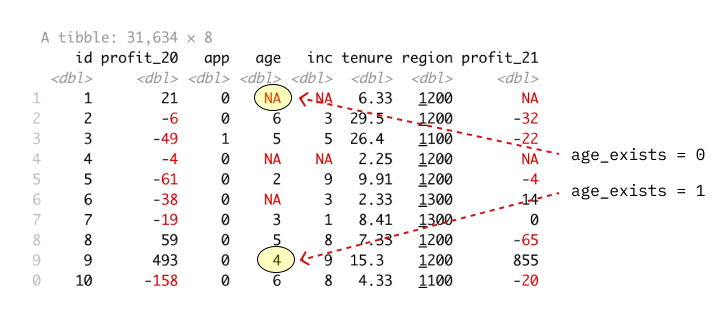
- Should we or shouldn’t we use the cases with missing data?
- What is the risk of omitting these cases?
Let’s test the influence
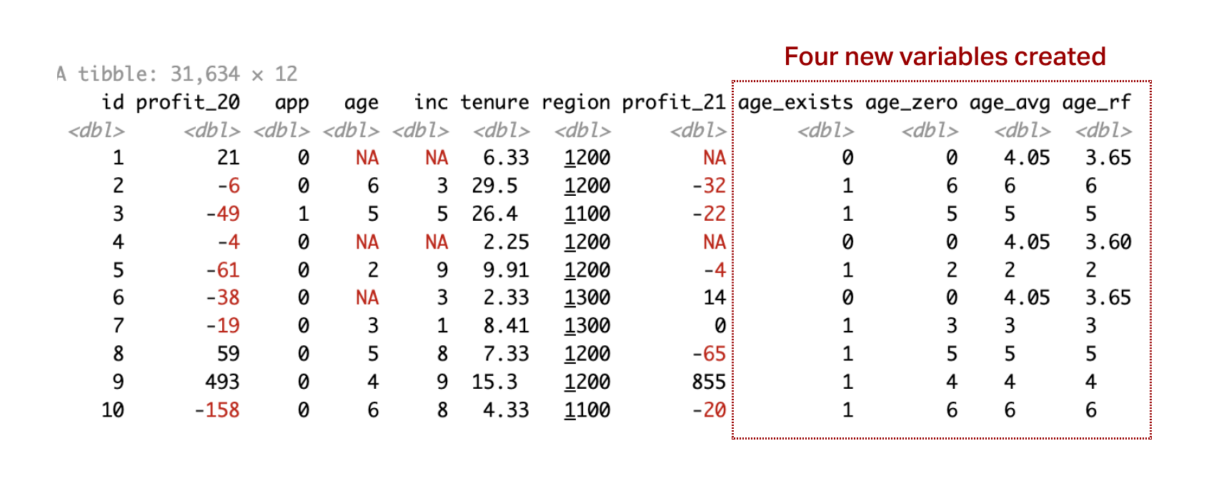
Create a new dummy variable age_exists that serves as a predictor. If it has a statistically significant impact on the results, we should be cautious about dropping missing values.
Influence of age
| Dependent variable: | ||
| profit_20 | ||
| App Only | App + Age Exists | |
| (1) | (2) | |
| app | 5.88 (4.69) | 3.56 (4.68) |
| age_exists | 52.14*** (3.48) | |
| Constant | 110.79*** (1.64) | 72.59*** (3.03) |
| Observations | 31,634 | 31,634 |
| R2 | 0.0000 | 0.01 |
| Adjusted R2 | 0.0000 | 0.01 |
| Residual Std. Error | 272.84 (df = 31632) | 271.88 (df = 31631) |
| F Statistic | 1.57 (df = 1; 31632) | 113.14*** (df = 2; 31631) |
| Note: | Significance: * p < 0.1, ** p < 0.05, *** p < 0.01 | |
Average or zero?
| Dependent variable: | ||
| profit_20 | ||
| Age Zero | Age Avg. | |
| (1) | (2) | |
| app | 19.65*** (4.69) | 19.65*** (4.69) |
| age_exists | -51.85*** (5.60) | 51.74*** (3.45) |
| age_zero | 25.60*** (1.09) | |
| age_avg | 25.60*** (1.09) | |
| Constant | 70.93*** (3.00) | -32.66*** (5.38) |
| Observations | 31,634 | 31,634 |
| R2 | 0.02 | 0.02 |
| Adjusted R2 | 0.02 | 0.02 |
| Residual Std. Error (df = 31630) | 269.52 | 269.52 |
| F Statistic (df = 3; 31630) | 262.12*** | 262.12*** |
| Note: | Significance: * p < 0.1, ** p < 0.05, *** p < 0.01 | |
What if we imputed the missing values?
Random forest
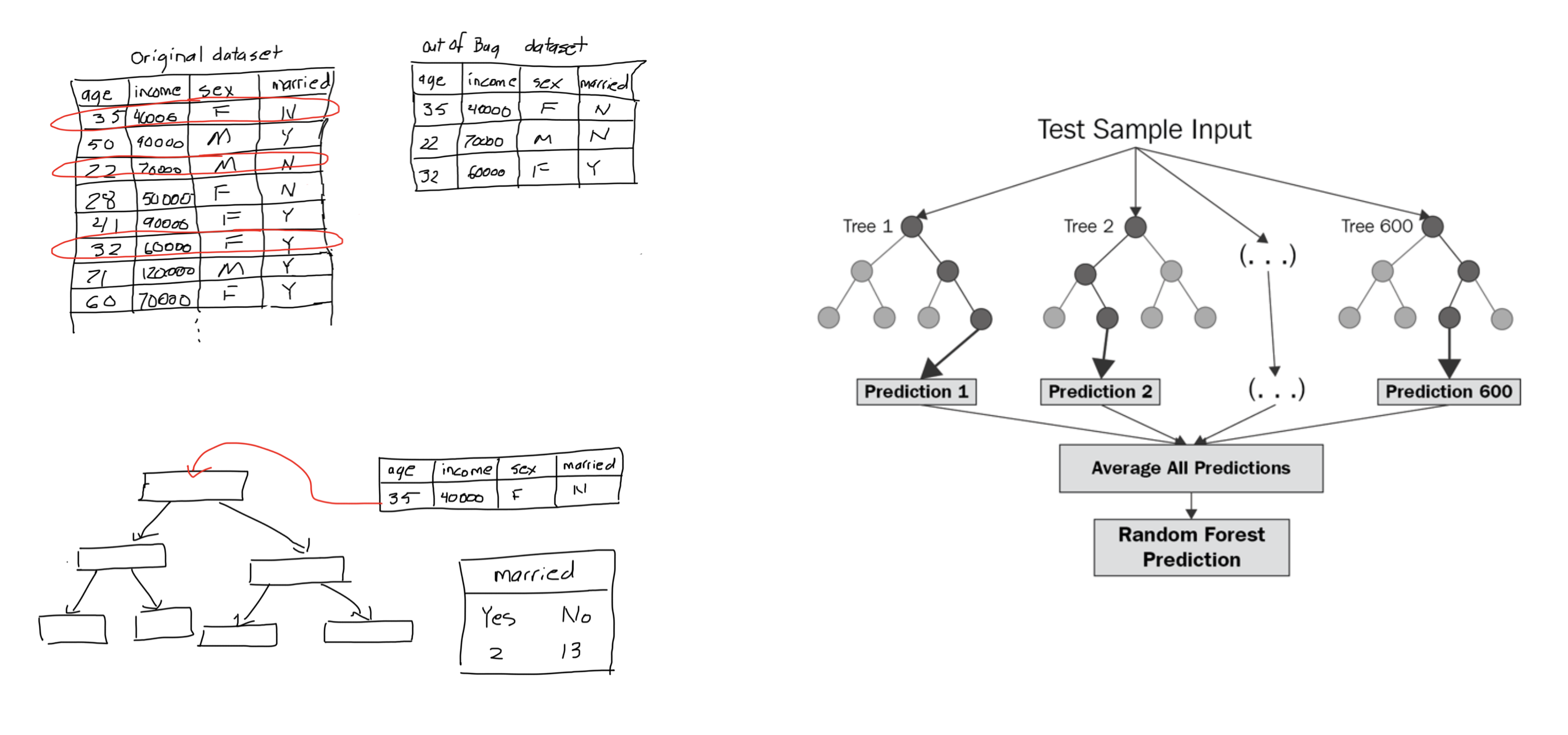
Using random forest
| Dependent variable: | |||
| profit_20 | |||
| Age Zero | Age Avg | Age RF | |
| (1) | (2) | (3) | |
| app | 19.65*** (4.69) | 19.65*** (4.69) | 27.39*** (4.69) |
| age_exists | -51.85*** (5.60) | 51.74*** (3.45) | 47.55*** (3.44) |
| age_zero | 25.60*** (1.09) | ||
| age_avg | 25.60*** (1.09) | ||
| age_rf | 30.63*** (1.07) | ||
| Constant | 70.93*** (3.00) | -32.66*** (5.38) | -49.80*** (5.22) |
| Observations | 31,634 | 31,634 | 31,634 |
| R2 | 0.02 | 0.02 | 0.03 |
| Adjusted R2 | 0.02 | 0.02 | 0.03 |
| Residual Std. Error (df = 31630) | 269.52 | 269.52 | 268.44 |
| F Statistic (df = 3; 31630) | 262.12*** | 262.12*** | 349.44*** |
| Note: | Significance: * p < 0.1, ** p < 0.05, *** p < 0.01 | ||
Back to the Data
Adding income
| Dependent variable: | ||
| profit_20 | ||
| App Only | App + Inc | |
| (1) | (2) | |
| app | 5.88 (4.69) | 16.25*** (4.64) |
| age_exists | 9.67 (8.20) | |
| age_rf | 31.92*** (1.06) | |
| inc_exists | 35.14*** (8.21) | |
| inc_rf | 21.80*** (0.74) | |
| Constant | 110.79*** (1.64) | -169.57*** (6.54) |
| Observations | 31,634 | 31,634 |
| R2 | 0.0000 | 0.06 |
| Adjusted R2 | 0.0000 | 0.06 |
| Residual Std. Error | 272.84 (df = 31632) | 264.77 (df = 31628) |
| F Statistic | 1.57 (df = 1; 31632) | 392.46*** (df = 5; 31628) |
| Note: | Significance: * p < 0.1, ** p < 0.05, *** p < 0.01 | |
How should we handle region data?
Adding region
| Dependent variable: | ||
| profit_20 | ||
| App Only | App + Region | |
| (1) | (2) | |
| app | 5.88 (4.69) | 15.87*** (4.64) |
| age_exists | 9.35 (8.20) | |
| age_rf | 32.11*** (1.06) | |
| inc_exists | 35.29*** (8.21) | |
| inc_rf | 21.28*** (0.76) | |
| region1200 | 14.12*** (5.14) | |
| region1300 | 6.06 (6.28) | |
| Constant | 110.79*** (1.64) | -179.03*** (7.71) |
| Observations | 31,634 | 31,634 |
| R2 | 0.0000 | 0.06 |
| Adjusted R2 | 0.0000 | 0.06 |
| Residual Std. Error | 272.84 (df = 31632) | 264.74 (df = 31626) |
| F Statistic | 1.57 (df = 1; 31632) | 281.74*** (df = 7; 31626) |
| Note: | Significance: * p < 0.1, ** p < 0.05, *** p < 0.01 | |
Final model
| Dependent variable: | ||
| profit_20 | ||
| App Only | App + All | |
| (1) | (2) | |
| app | 5.88 (4.69) | 16.01*** (4.61) |
| age_exists | 2.33 (8.15) | |
| age_rf | 21.73*** (1.17) | |
| inc_exists | 32.20*** (8.16) | |
| inc_rf | 19.86*** (0.75) | |
| region1200 | 15.52*** (5.10) | |
| region1300 | 6.17 (6.24) | |
| tenure | 4.07*** (0.20) | |
| Constant | 110.79*** (1.64) | -164.72*** (7.69) |
| Observations | 31,634 | 31,634 |
| R2 | 0.0000 | 0.07 |
| Adjusted R2 | 0.0000 | 0.07 |
| Residual Std. Error | 272.84 (df = 31632) | 262.97 (df = 31625) |
| F Statistic | 1.57 (df = 1; 31632) | 303.24*** (df = 8; 31625) |
| Note: | Significance: * p < 0.1, ** p < 0.05, *** p < 0.01 | |
What about 2021 profitability?
Back to demographics
| Dependent variable: | |
| profit_21 | |
| demographics | 47.53*** (5.98) |
| Constant | 106.86*** (5.34) |
| Observations | 26,396 |
| R2 | 0.002 |
| Adjusted R2 | 0.002 |
| Residual Std. Error | 389.54 (df = 26394) |
| F Statistic | 63.19*** (df = 1; 26394) |
| Note: | Significance: * p < 0.1, ** p < 0.05, *** p < 0.01 |
A better model
| Dependent variable: | |
| profit_21 | |
| app | 18.77*** (5.84) |
| region1200 | 15.10** (6.55) |
| region1300 | 11.21 (8.15) |
| tenure | 0.92*** (0.23) |
| profit_20 | 0.83*** (0.01) |
| Constant | 19.82*** (6.70) |
| Observations | 26,396 |
| R2 | 0.36 |
| Adjusted R2 | 0.36 |
| Residual Std. Error | 312.04 (df = 26390) |
| F Statistic | 2,968.07*** (df = 5; 26390) |
| Note: | Significance: * p < 0.1, ** p < 0.05, *** p < 0.01 |
What to do next?
- What about retention? Can a case be made that the app creates value by making customers more sticky?
- Create a new regression model using a new
retaineddependent variable.
(Hint: You can calculate based on whether or not value is present inprofit_21or not.) - Compare results between linear regression and logistic regression.