Working with Behavioral Data

Overview

Learning about customers through the data collected through business and relationship management systems.

Presented by:
Larry Vincent,
Professor of the Practice, Marketing

Presented to:
MKT 512
October 22, 2025

Behavioral data and customer profiling

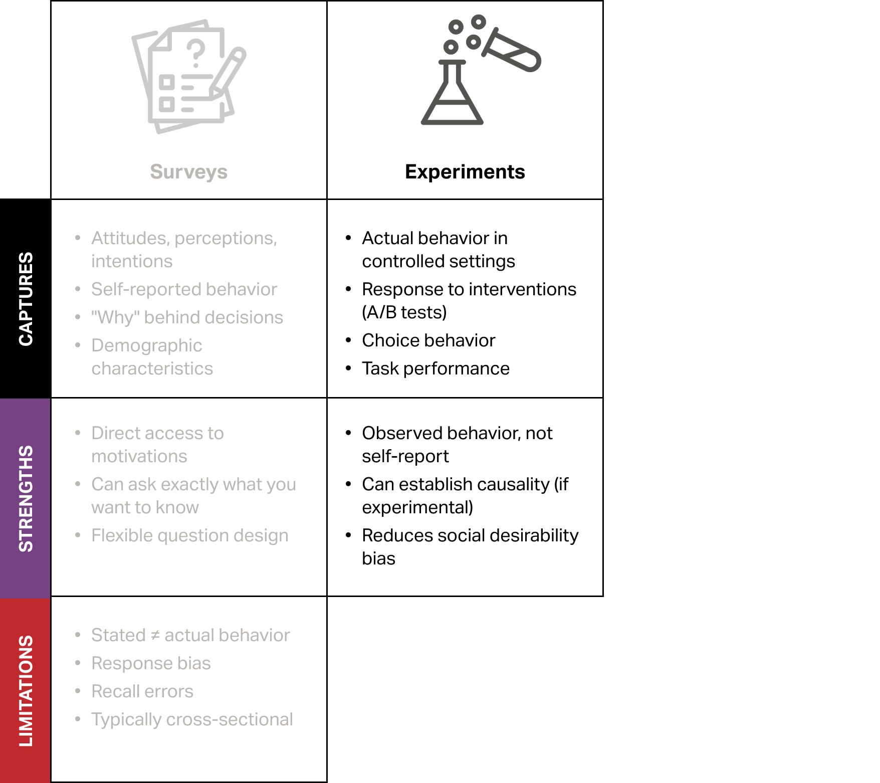
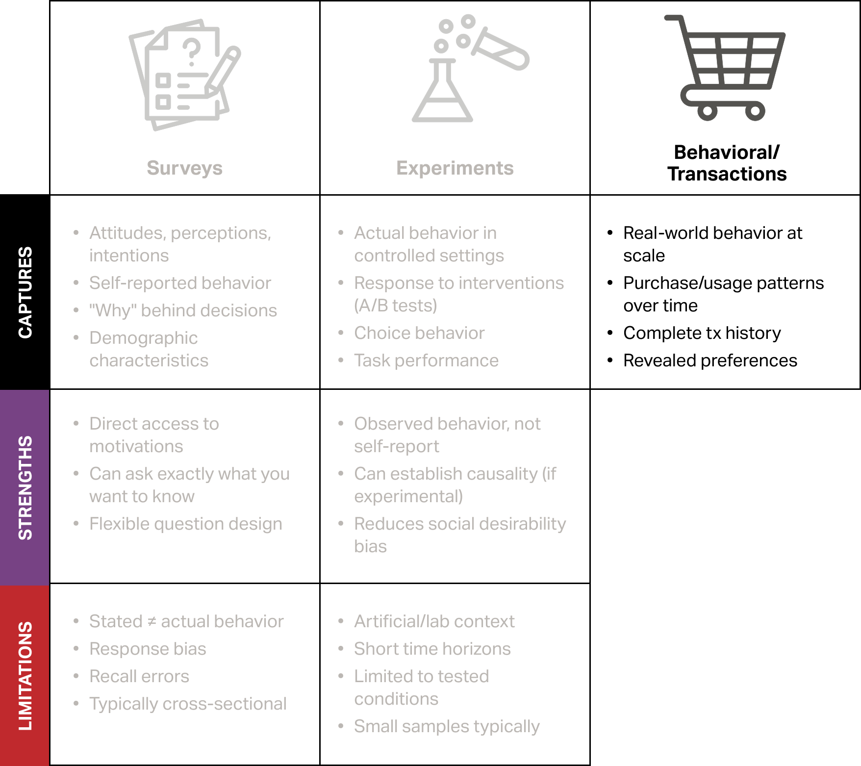
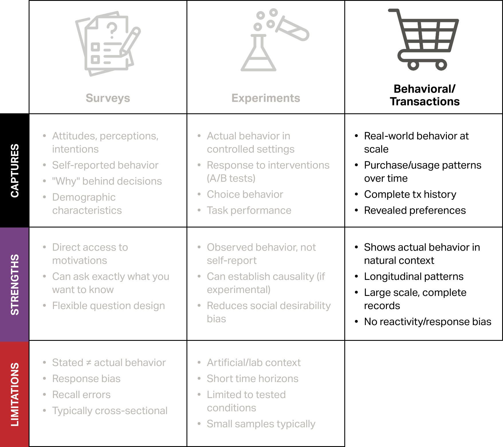
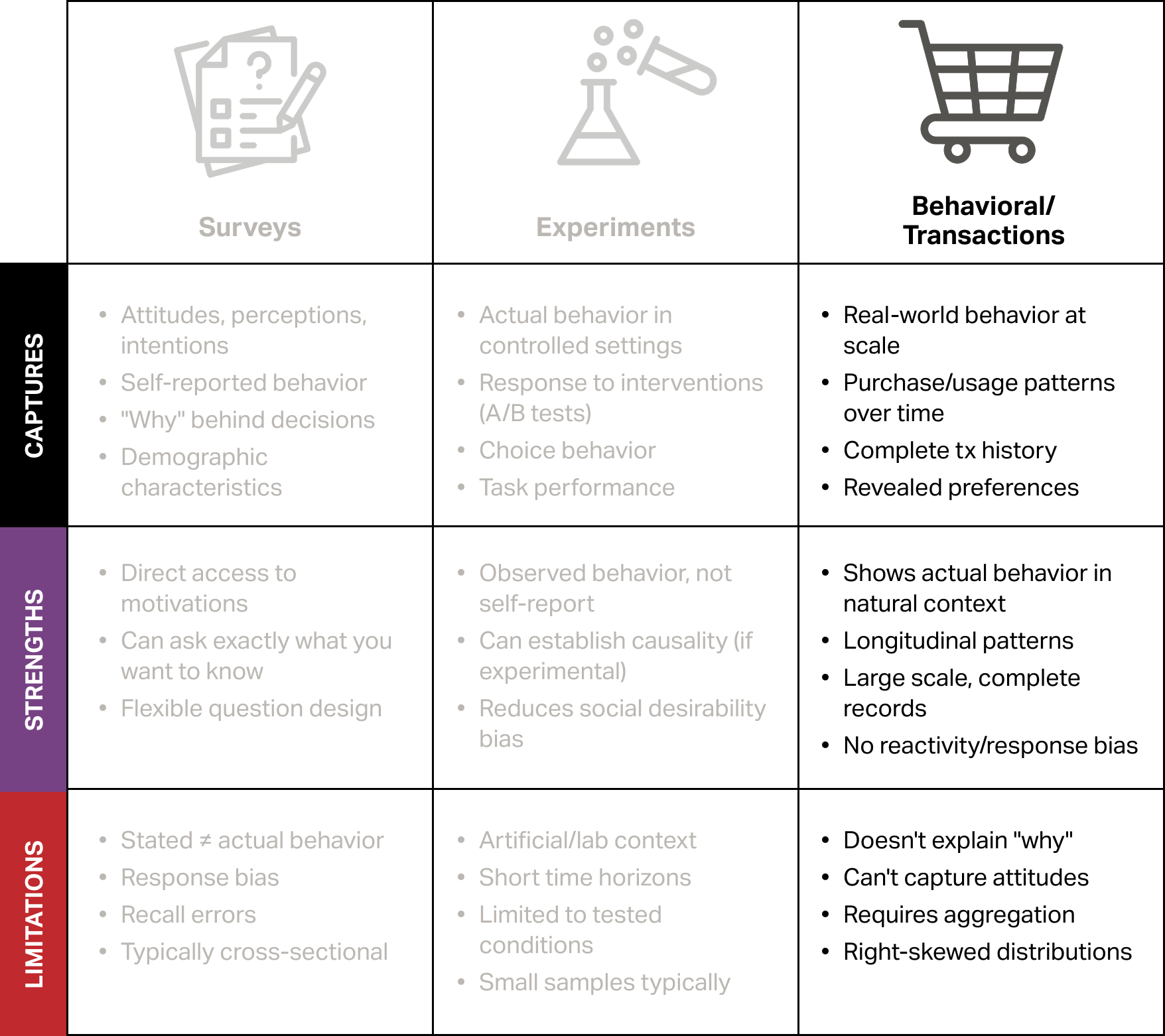
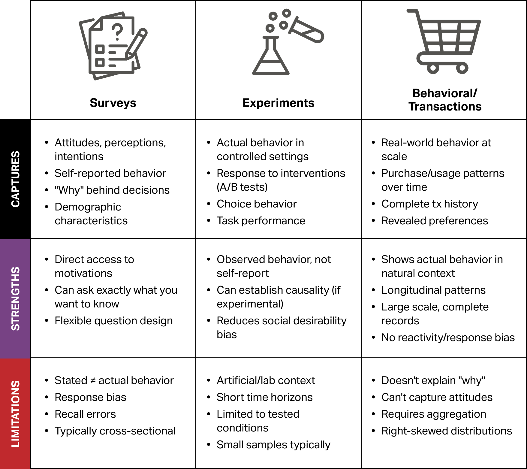
Comparing options

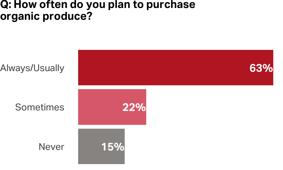
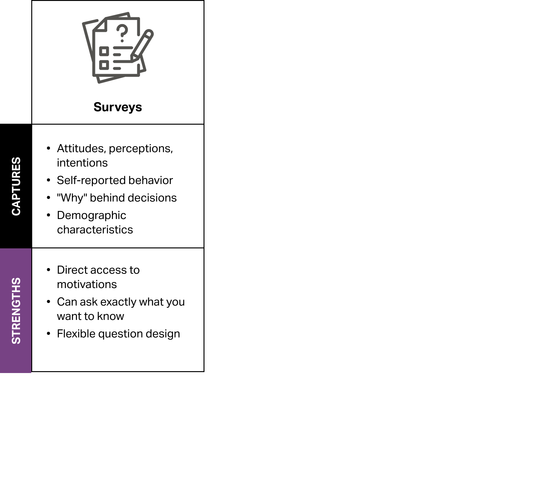
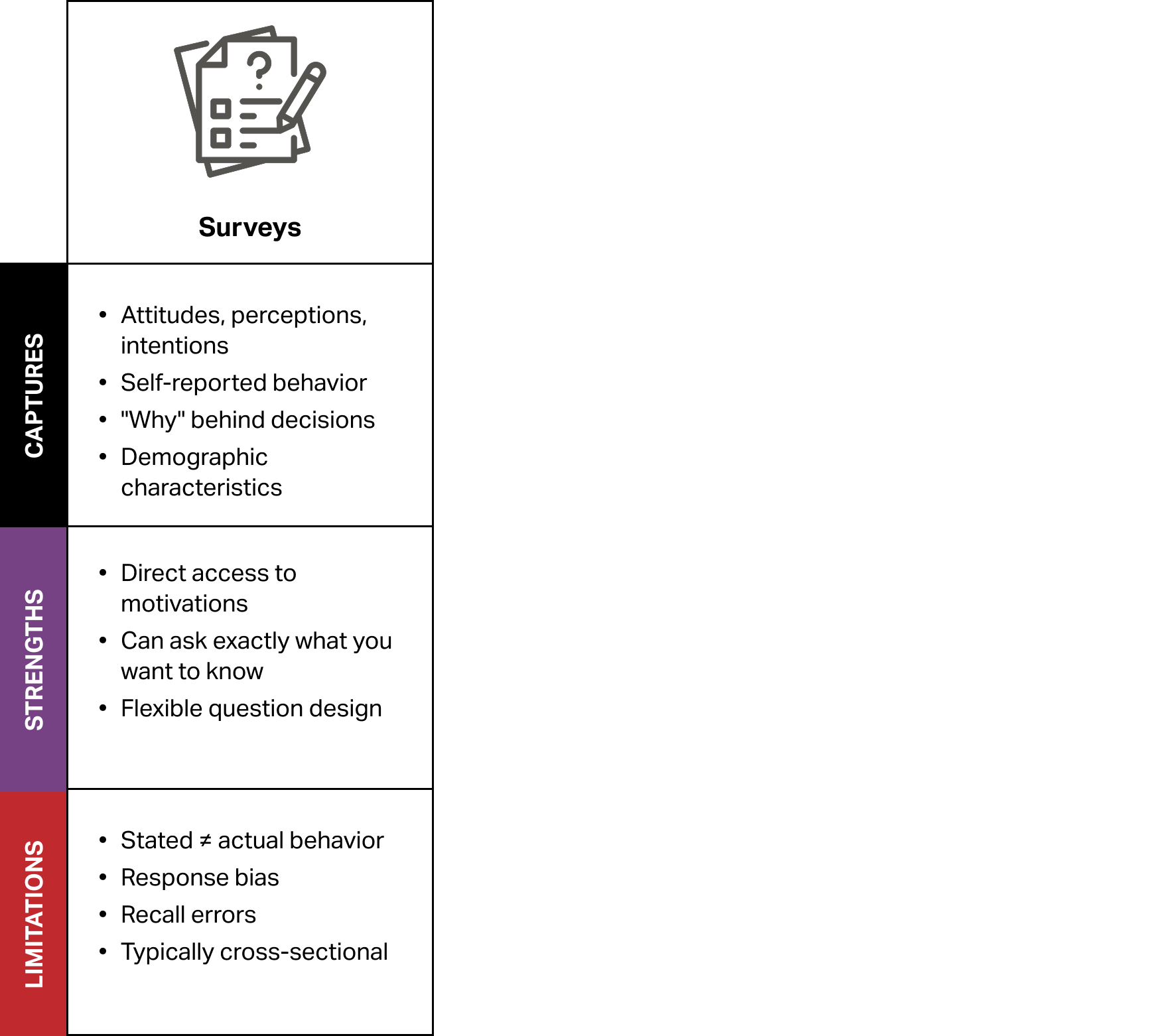
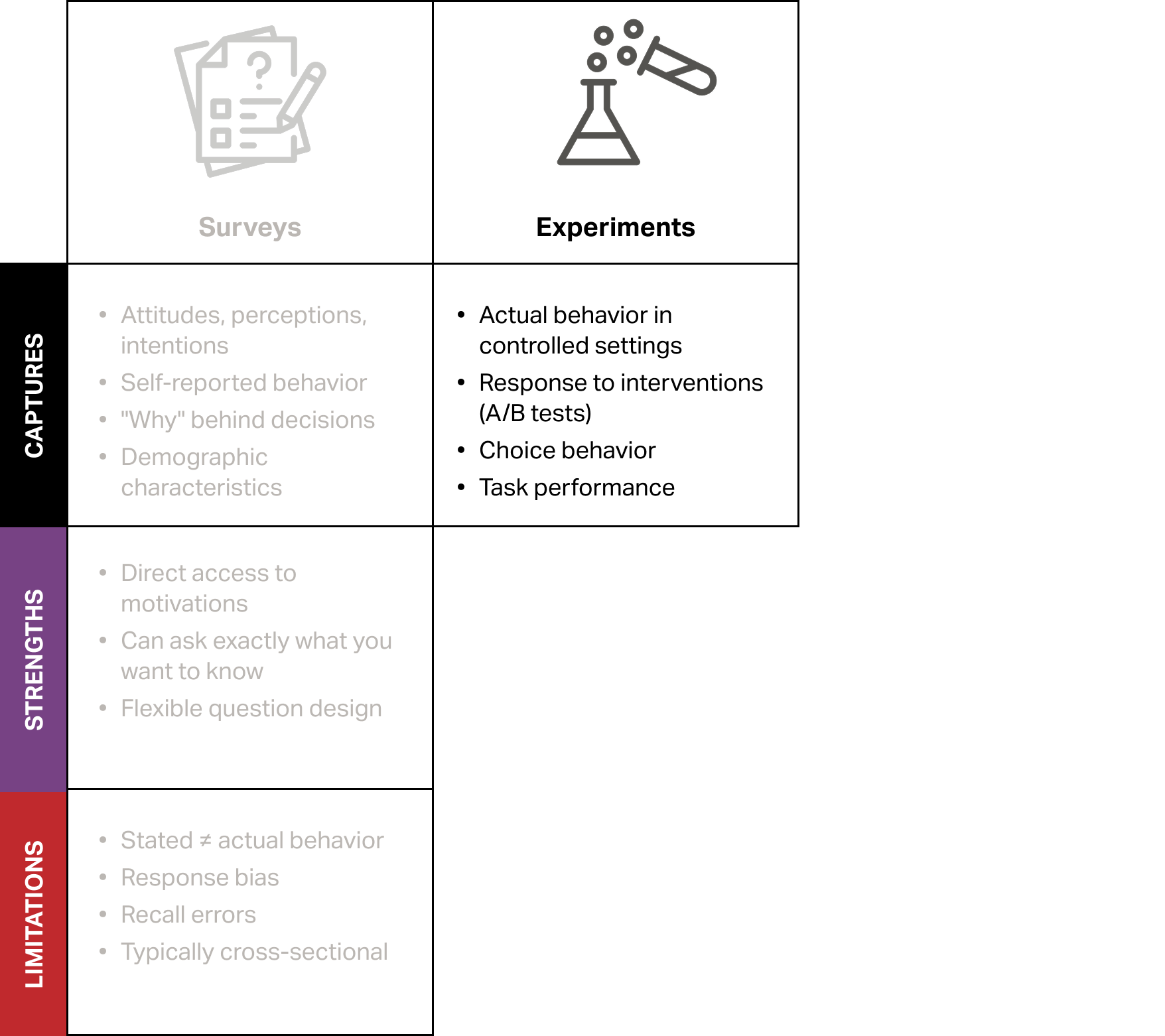
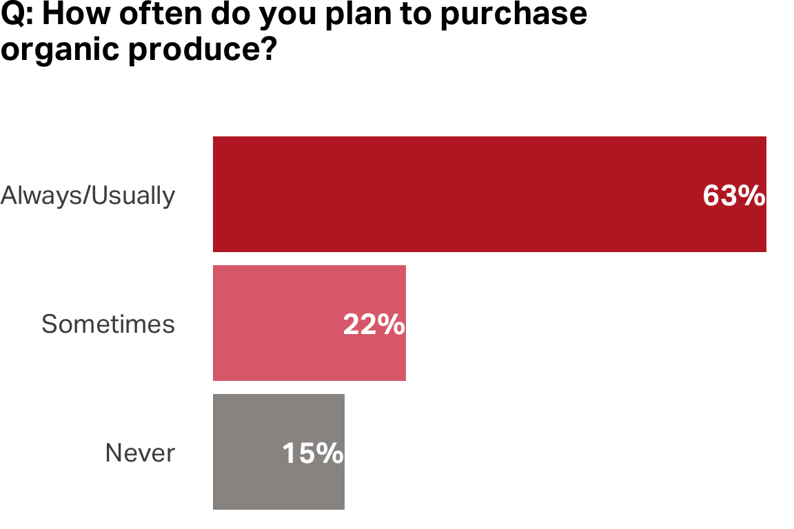
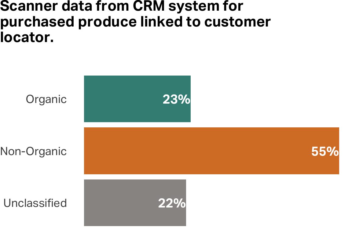
Stated preferences vs. revealed

Stated preferences vs. revealed

Most used behavior metrics

Recency–How recently have they engaged with us?

Most used behavior metrics

Recency–How recently have they engaged with us?
Frequency–How often do they tend to engage with us?

Most used behavior metrics

Recency–How recently have they engaged with us?
Frequency–How often do they tend to engage with us?
Velocity–Is their behavior accelerating, declining or stable?

Most used behavior metrics

Recency–How recently have they engaged with us?
Frequency–How often do they tend to engage with us?
Velocity–Is their behavior accelerating, declining or stable?
Monetary–How much do they typically spend or how much have they spent since originating?

Sample data

We will be working with a synthetic data set for a fictional company. The data set has four columns, transaction_id, customer_id, transaction_date, and transaction_amount.

File: customer-transactions-data.csv

transaction_id	customer_id	transaction_date	transaction_amount
TXN0000001	CUST04313	2023-01-01	118.43
TXN0000002	CUST00041	2023-01-02	111.25
TXN0000003	CUST00152	2023-01-02	118.83
TXN0000004	CUST00293	2023-01-02	54.96
TXN0000005	CUST00341	2023-01-02	139.38
TXN0000006	CUST00498	2023-01-02	83.58

Transforming to customer data

# Set a cutoff point--here it's the day after the last transaction date
ANALYSIS_DATE <- as_date("2025-10-01")

# Group by customer to calculate customer behaviors
customers_df <- df |> 
  group_by(customer_id) |> 
  summarise(
    last_transaction = max(transaction_date),
    recency = as.numeric(ANALYSIS_DATE - last_transaction),
    frequency = n(),
    monetary = sum(transaction_amount),
    avg_tx = mean(transaction_amount)
  )

Transforming to customer data

# Set a cutoff point--here it's the day after the last transaction date
ANALYSIS_DATE <- as_date("2025-10-01")

# Group by customer to calculate customer behaviors
customers_df <- df |> 
  group_by(customer_id) |> 
  summarise(
    last_transaction = max(transaction_date),
    recency = as.numeric(ANALYSIS_DATE - last_transaction),
    frequency = n(),
    monetary = sum(transaction_amount),
    avg_tx = mean(transaction_amount)
  )

# A tibble: 6 × 6
  customer_id last_transaction recency frequency monetary avg_tx
  <chr>       <date>             <dbl>     <int>    <dbl>  <dbl>
1 CUST00001   2025-01-01           273         4     318.   79.5
2 CUST00002   2025-07-15            78         4     279.   69.8
3 CUST00003   2025-09-26             5        18    1952.  108. 
4 CUST00004   2025-09-06            25        19    1728.   90.9
5 CUST00005   2025-09-11            20         8     787.   98.4
6 CUST00006   2025-09-24             7        66   14967.  227.

Recency

The number of days (or time period) since a customer’s last transaction or interaction.

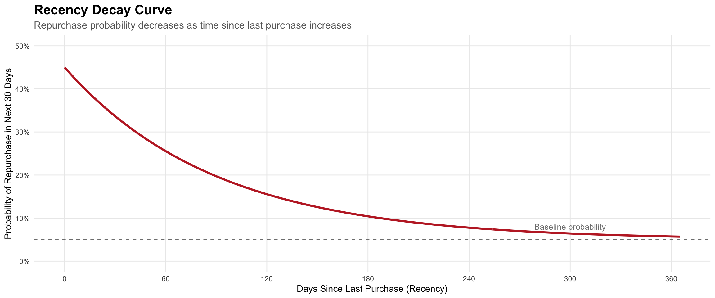
Decay curve

Customer repurchase probability decays over time, though the rate varies dramatically by category (fast-moving consumer goods decay quickly; durable goods like appliances show flat patterns).

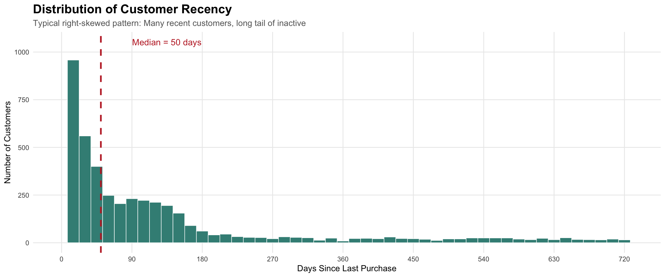
Analyzing recency patterns

Notice the concentration of customers with recent purchases (left side) and the long tail of inactive customers extending to the right—this pattern suggests most customers are engaged, but you have a significant inactive segment requiring re-engagement strategies.

Predictive Models

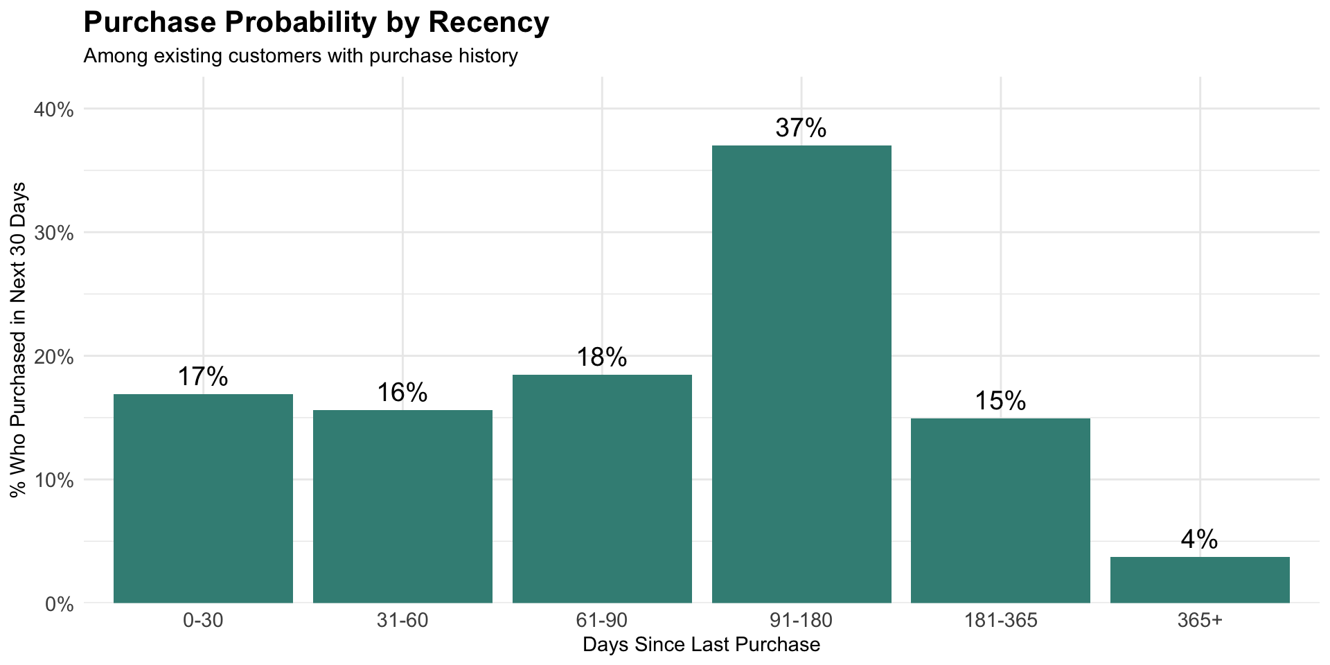
Recency scores can help us understand common patterns and probability of purchase within certain windows. These probabilities can be used to optimize marketing mix decisions.

Recency needs context

Two customers with same recency (30 days)

Customer A: Second purchase in < 30 days
→ Promising new customer

Customer B: Only purchase in 2 years
→ At-risk, declining customer

We need additional context

How often do they engage?
How much do they spend?
Are they accelerating or declining?

With this context, you can then develop strategy.

Winback lapsing and at-risk customers or take the win but don’t waste resources on inconsistent or opportunistic customers
Incentivize return visit from new customer or target for special offer/reward

Next: Frequency as the second behavioral dimension

Frequency

The number of transactions or interactions a customer has made within a specified time period.

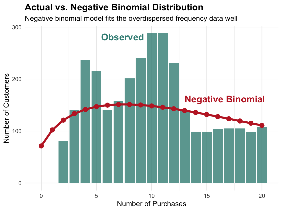
Frequency as count data

Frequency is count data (integers ≥ 0), which requires specialized statistical methods. When the variance exceeds the mean (overdispersion) or there’s excess zeros, negative binomial or zero-inflated models are more appropriate than standard linear regression.

Properties of Count Data:

Only non-negative integers (0, 1, 2, 3…)
Cannot be averaged meaningfully
Variance often increases with mean
Excess zeros common (many one-time purchasers)

Statistical approaches:

Poisson regression (if mean ≈ variance)
Negative binomial (if overdispersed)
Zero-inflated models (if excess zeros)

Frequency is context-dependent

What constitutes “high frequency” varies dramatically by business model and product category. A metric that signals engagement in one industry may indicate completely different behavior in another.

Business Model	High Frequency	Interpretation
Coffee Shop	20+ visits/month	Daily regular
Grocery Store	2-3 visits/week	Weekly shopper
E-commerce Fashion	8-12 orders/year	Fashion enthusiast
SaaS (B2B)	Daily logins	Power user
Luxury Auto	1 purchase/5 years	Repeat customer (rare!)
Streaming Service	Daily usage	Core subscriber

Count data requires care

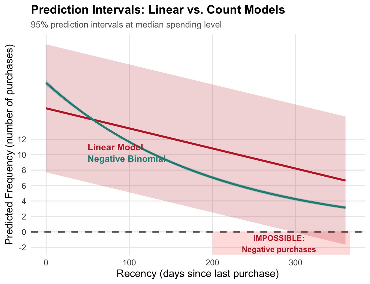
Linear regression on count data produces nonsensical prediction intervals that include negative frequencies—an impossibility for count data.

# Wrong approach: Linear model
lm_model <- lm(frequency ~ recency + monetary,
               data = customers_df)

# Prediction intervals
predict(lm_model, interval = "prediction")

# Right approach: Negative binomial
# using glm.nb function from MASS package
nb_model <- glm.nb(frequency ~ recency + monetary,
                   data = customers_df)

Key Problem: Linear model assumes constant variance and normal errors—both violated with count data.

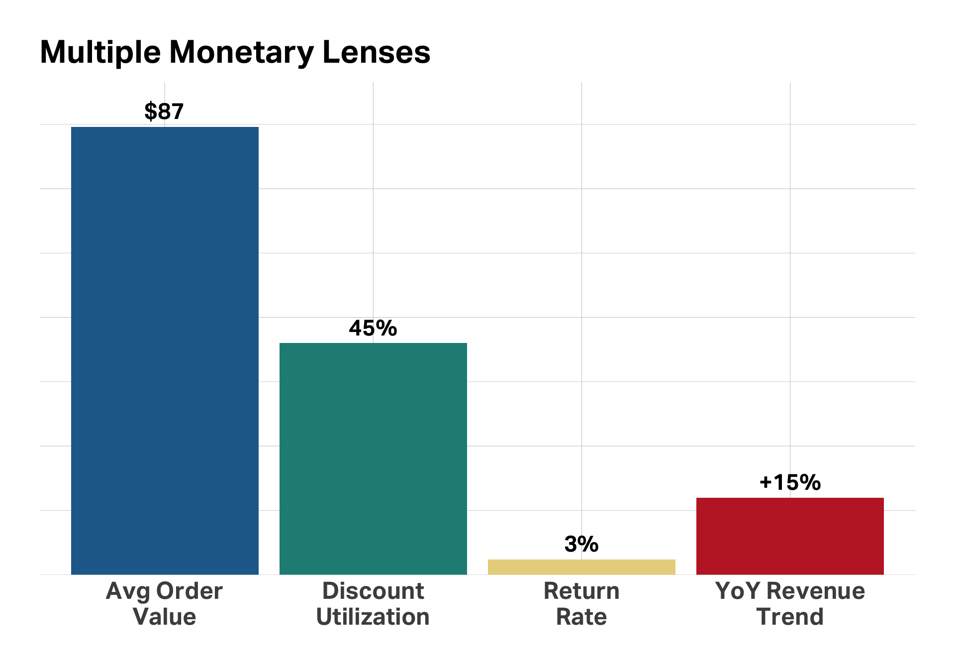
Monetary value

The financial dimension of customer behavior, revealing spending patterns, preferences, and relationship depth beyond simple revenue totals

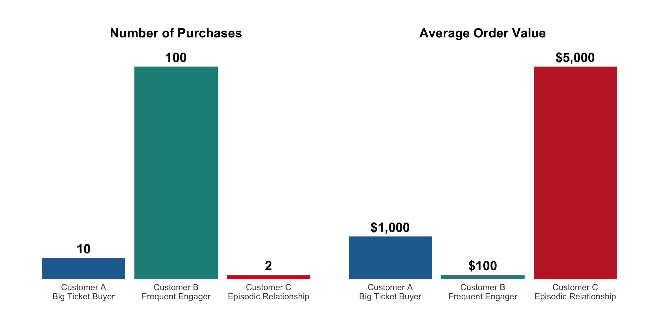
Beyond the total

Customer Profile

Lifetime Spend:
$5,240

Transactions:
60

Time Period:
36 months

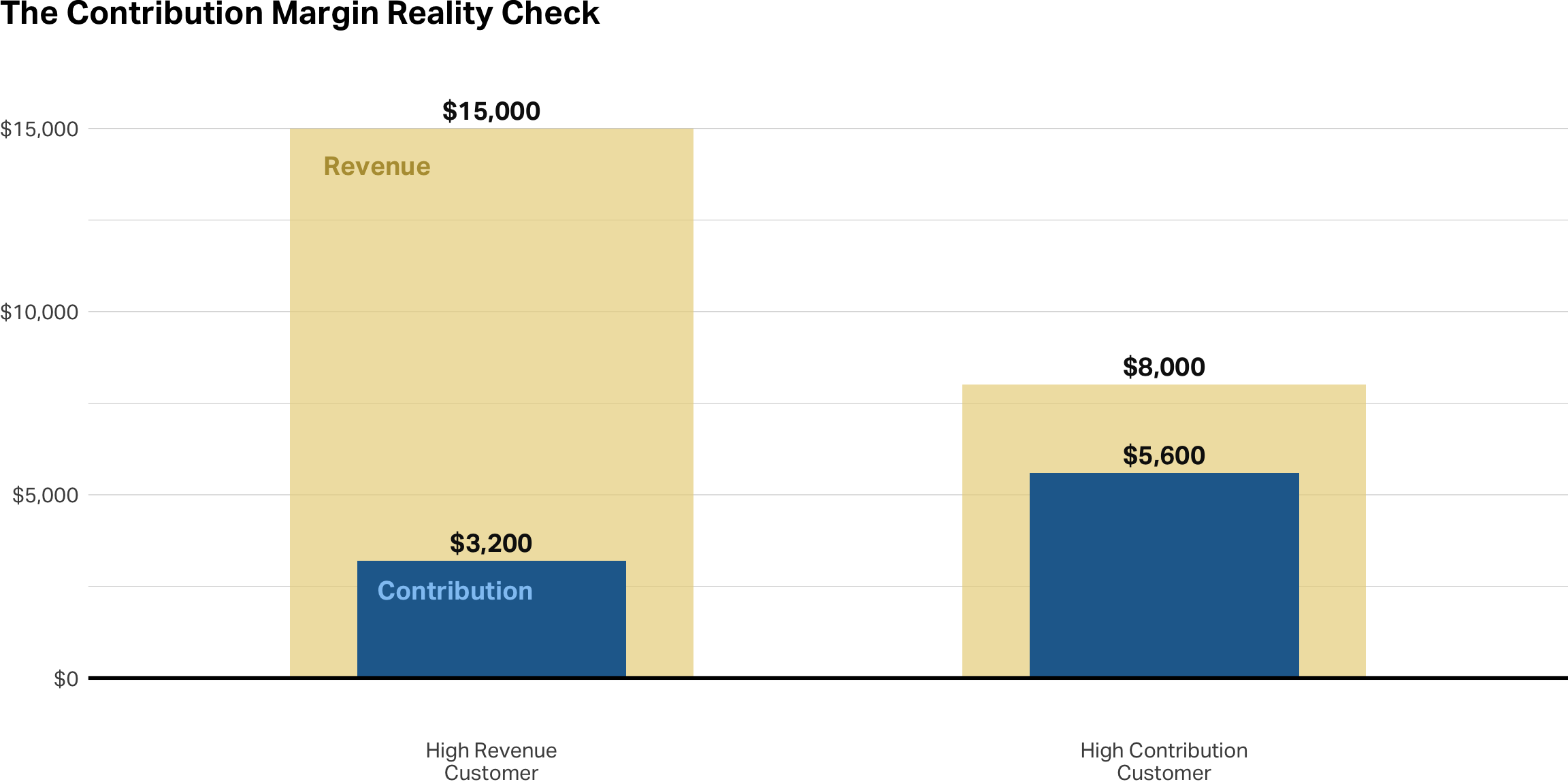
All revenue is not equal

Identical revenue ($10,000), completely different relationships and strategies needed

Revenue ≠ Value

Behavioral patterns (discount seeking, returns) directly impact true value

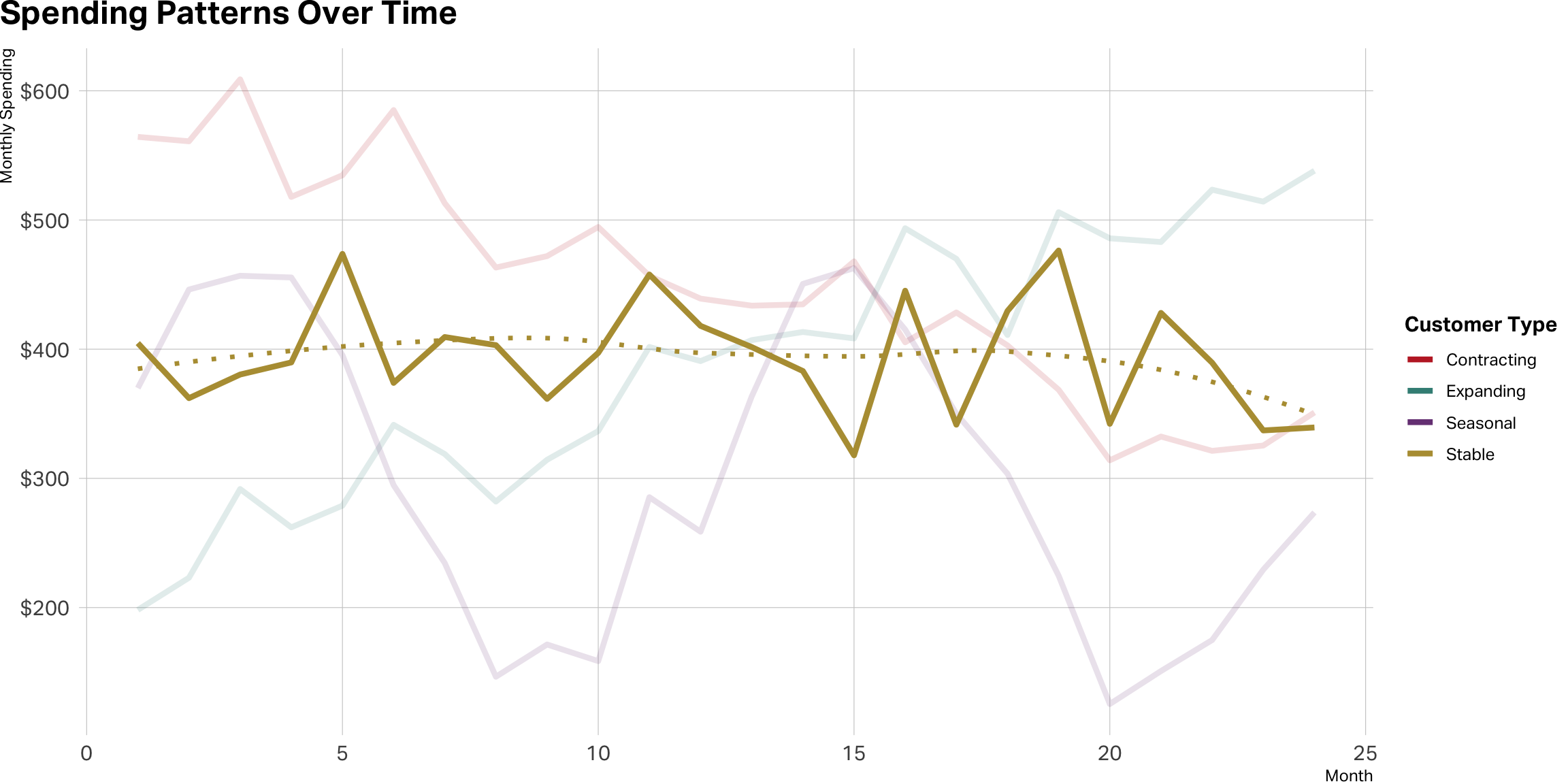
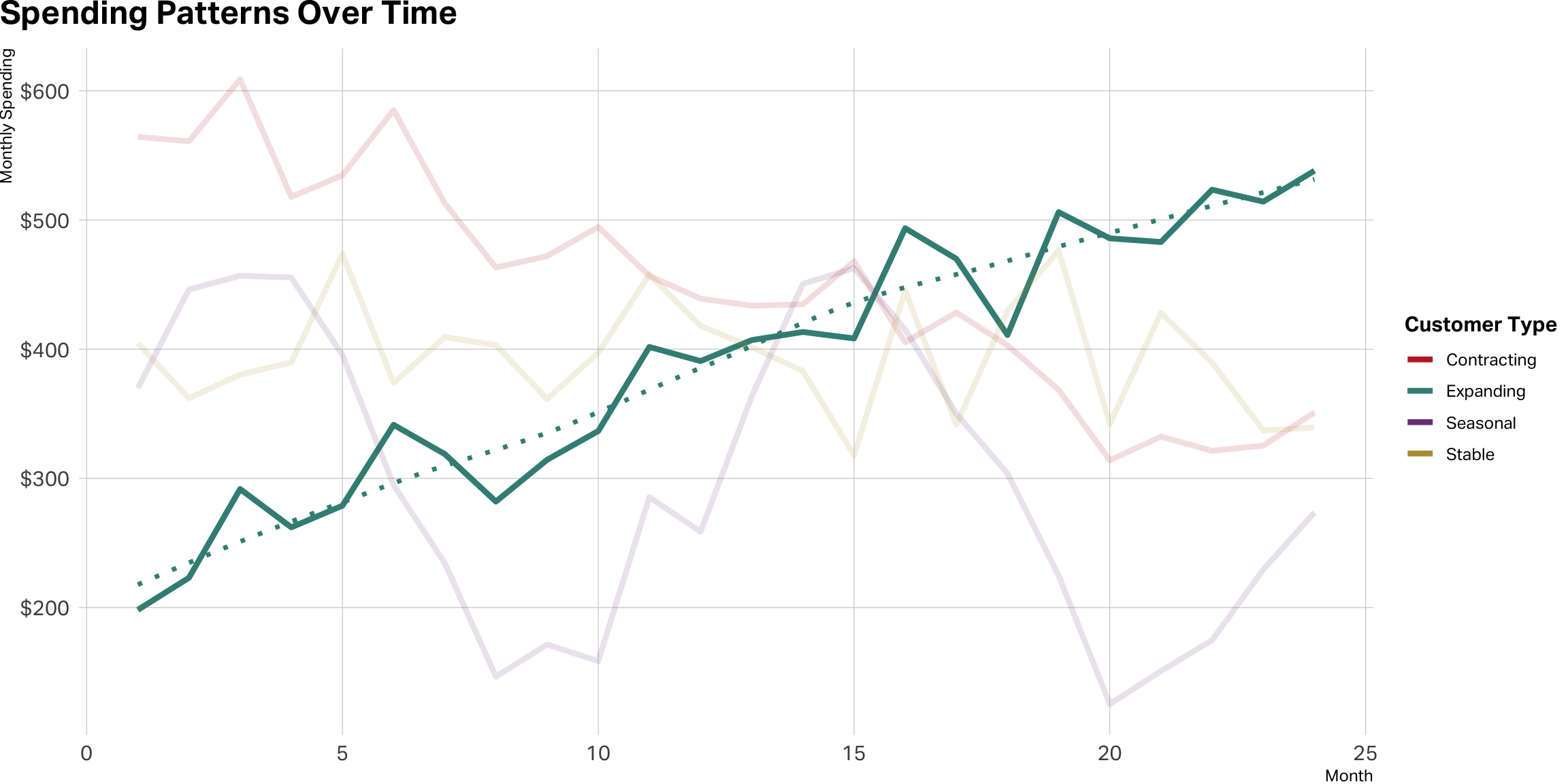
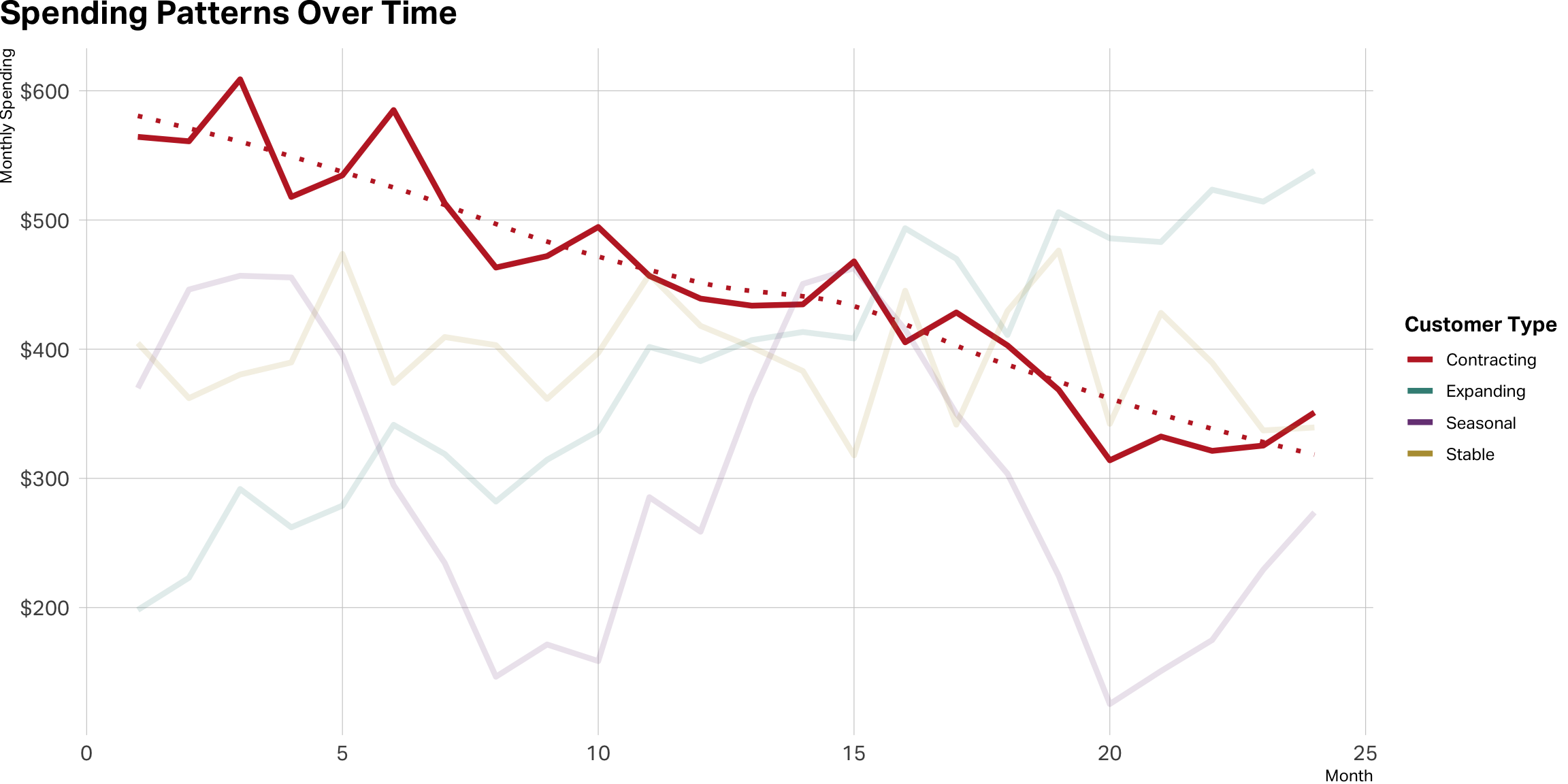
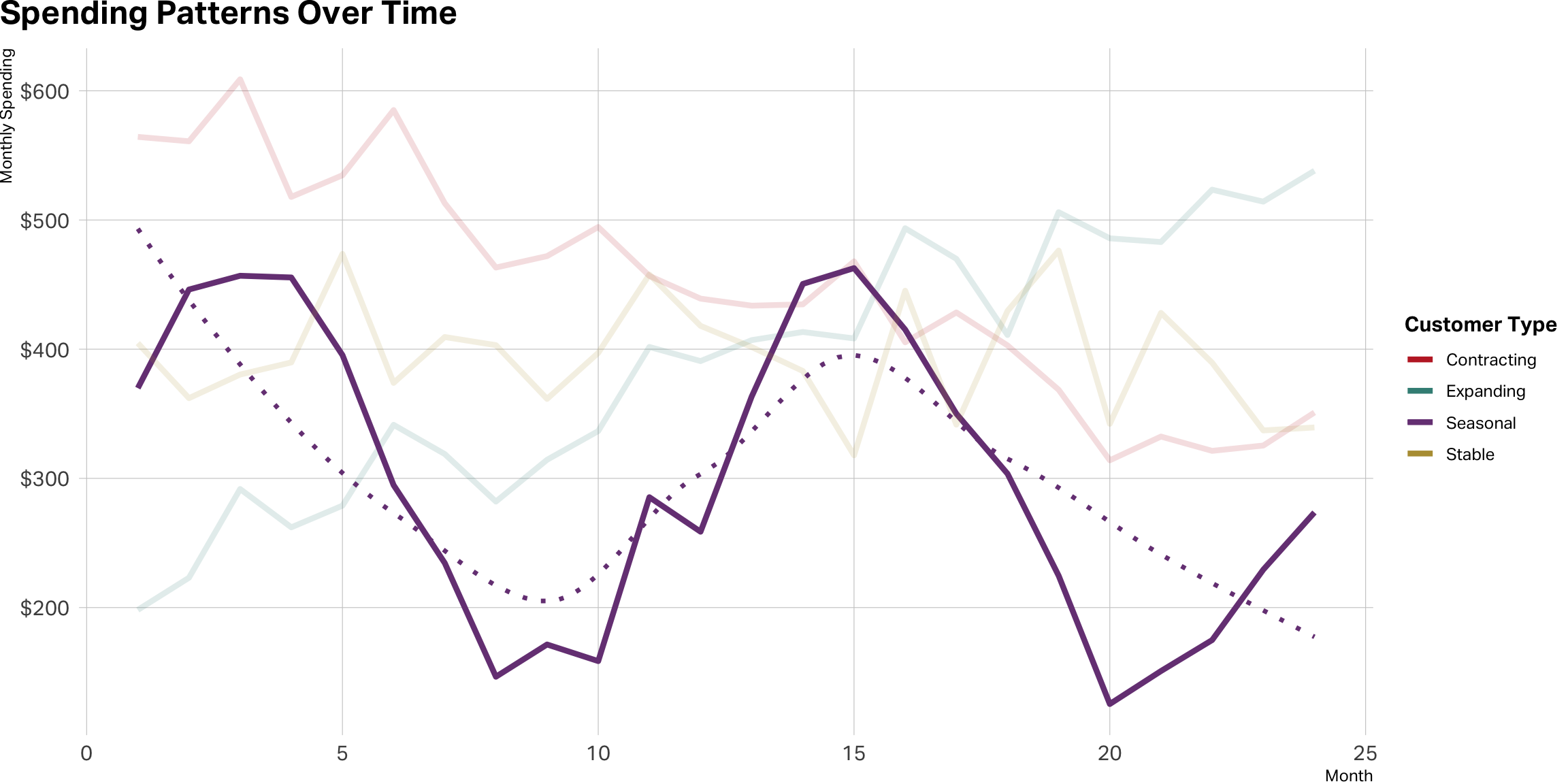
Stable is not a straight line

Lean in on expansion

Contraction is a red flag

Seasonal cases can be tricky

Takeaway

Monetary metrics are behavioral signals
Patterns reveal relationship depth, preferences, and trajectory
Understanding how customers spend is as important as how much

Next: Velocity — quantifying behavioral change over time

Velocity

The rate of change in customer behavior over time, revealing whether engagement is accelerating, decelerating, or stable.

Velocity takes many forms

Context determines which velocity metric matters most for your business

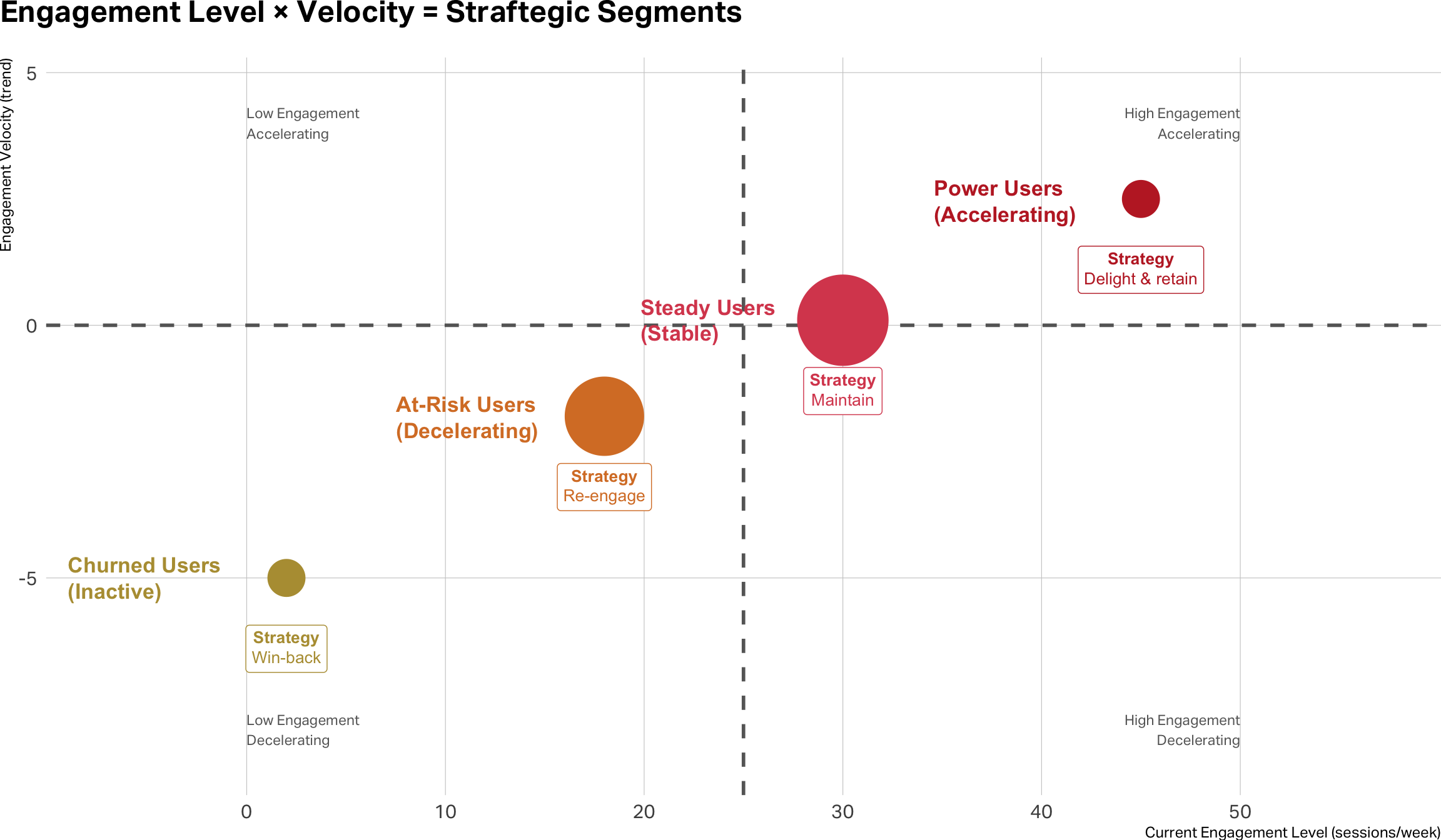
Engagement Velocity

Login frequency trends
Content consumption patterns
Feature usage intensity
Session duration changes

Transaction Velocity

Purchase frequency changes
Time between orders
Repeat purchase acceleration

Spending Velocity

Average order value trends
Basket size growth
Wallet share expansion

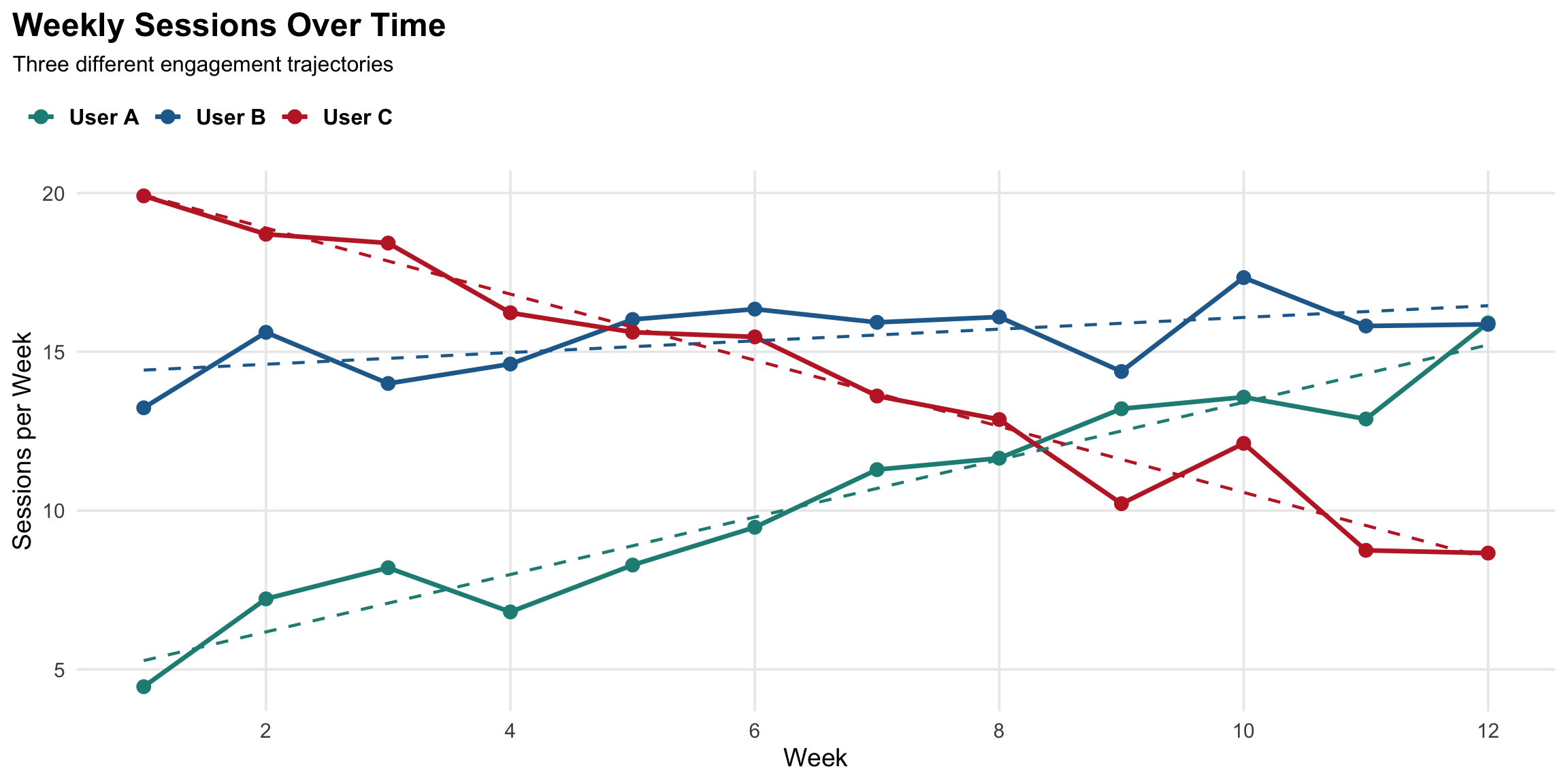
Measuring engagement velocity

Calculating velocity

Simple approach

Period-over-period change

Week 1-4 average: 8 sessions
Week 9-12 average: 14 sessions

Velocity = +75% growth

✓ Easy to calculate
✓ Intuitive to interpret
⚠️ Sensitive to outliers

Regression approach

Slope of trend line

model <- lm(sessions ~ week, 
            data = user_data)
velocity <- coef(model)["week"]
# Positive = accelerating
# Negative = decelerating

✓ Accounts for all data
✓ Less noise
✓ Statistical significance testing

Patterns vs. implications

Real-world velocity metrics

The specific metric varies, but the concept is universal: behavior change over time

Streaming (Netflix, Spotify)

Hours streamed per week
Content starts per session
Days active per month
Genre exploration rate

SaaS Products

Daily/weekly active users
Feature adoption rate
Time in application
Collaboration events

E-commerce

Days between purchases
Browse-to-buy conversion
Category expansion
Cart value trajectory

Social Platforms

Posts/comments per week
Connection growth rate
Engagement with content
Time on platform

Takeaway

Velocity adds the temporal dimension
Static metrics show where customers are → Velocity shows
where they’re going
Early warning system for churn and expansion opportunities

Next: Bringing it together with RFM scoring

RFM Analysis

Combining recency, frequency, and monetary metrics to create actionable customer segments for strategic marketing decisions.

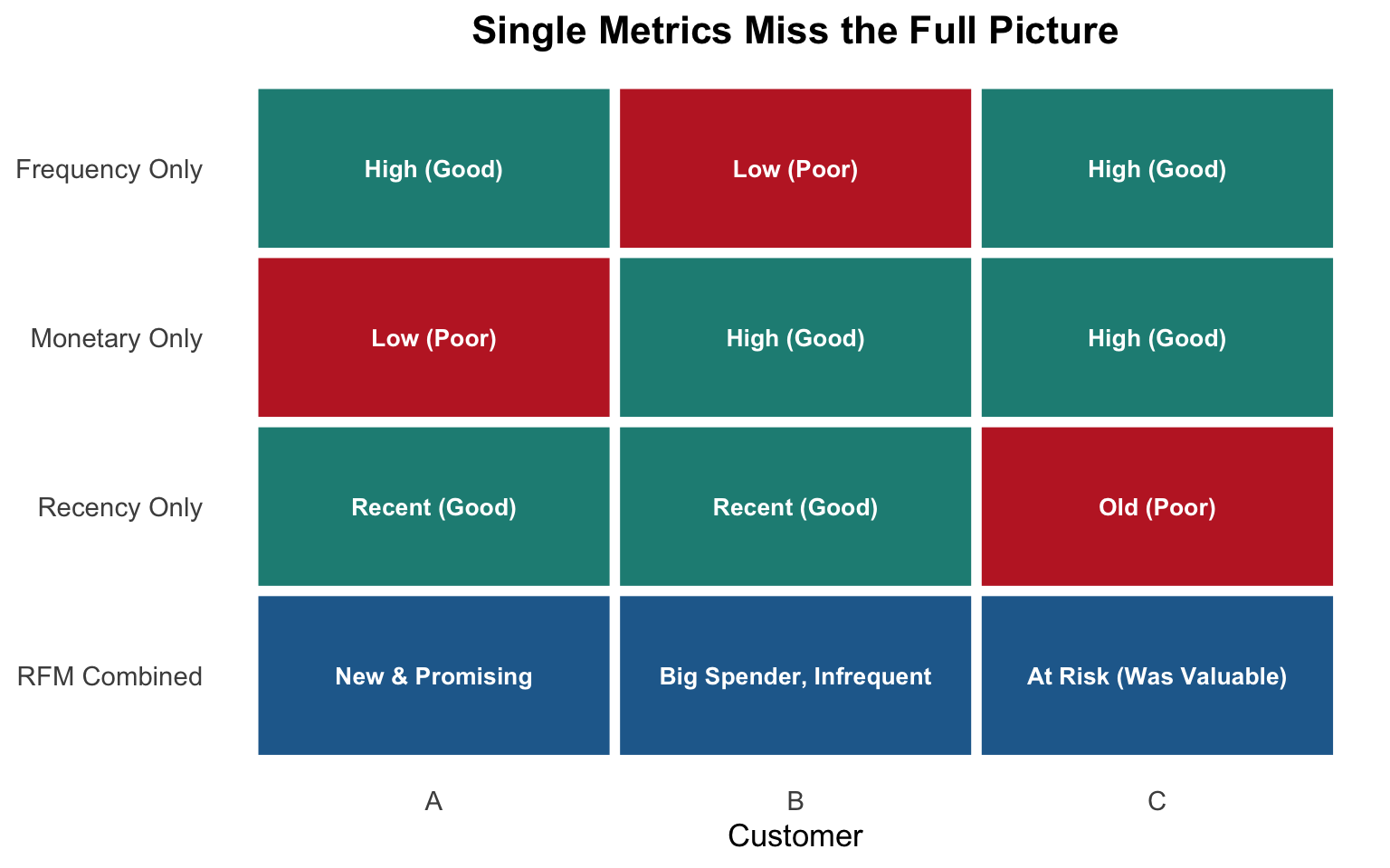
Why combine R, F, and M?

Each dimension alone provides incomplete information. Combined, they reveal distinct customer archetypes requiring different strategies.

Recency alone:
Can’t distinguish new customers from declining ones

Frequency alone:
Misses spending power and engagement timing

Monetary alone:
Ignores relationship trajectory and engagement patterns

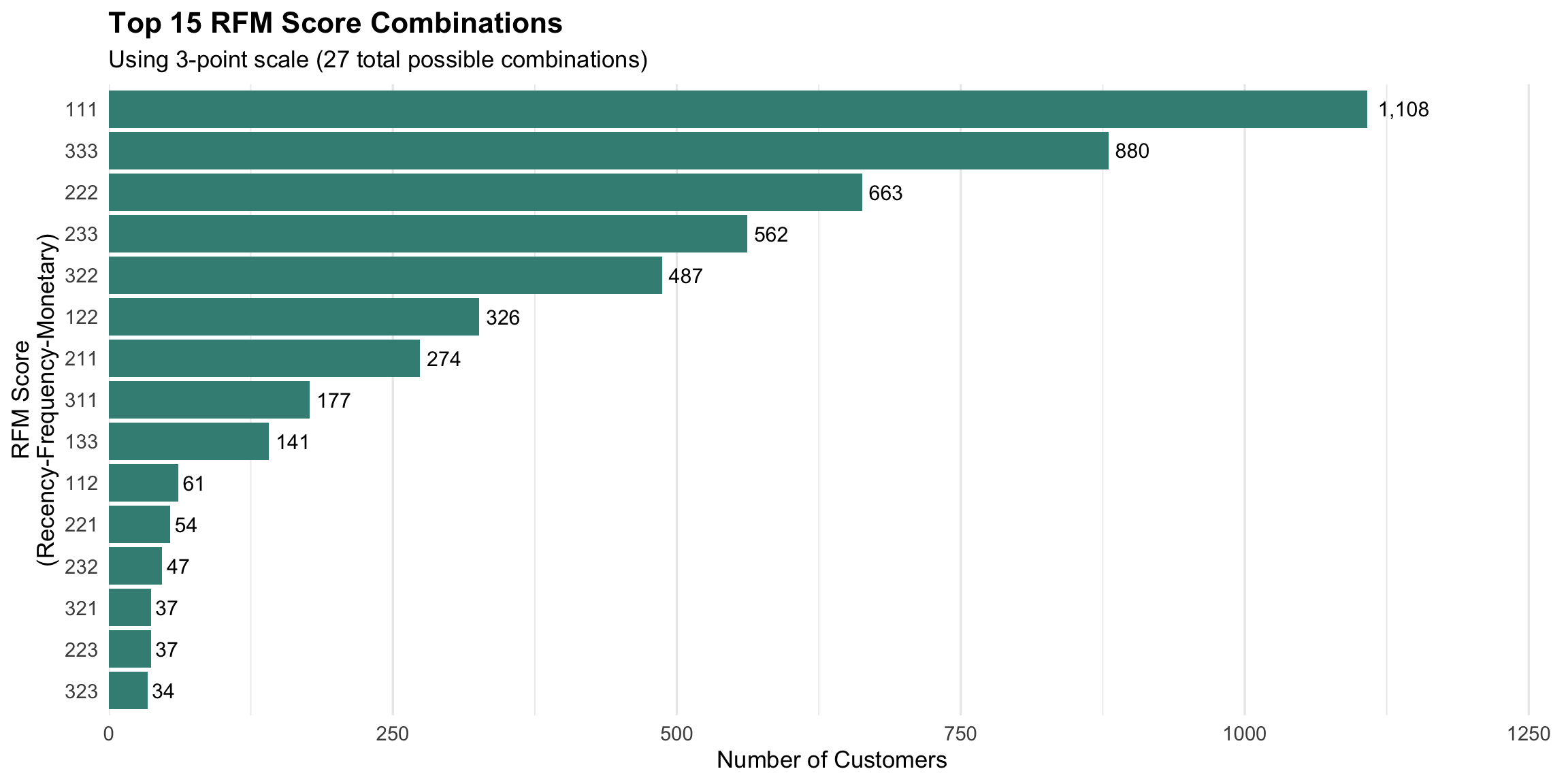
Creating RFM scores

Customers are ranked and divided into groups (typically 3-5) for each dimension, creating a composite score that enables segmentation.

Scoring Approaches:

Quintiles (5-point scale) - Divide customers into 5 equal groups - Score 5 = top 20%, Score 1 = bottom 20% - Creates 125 possible combinations (5³) - More granular, harder to interpret

Tertiles (3-point scale) - Divide customers into 3 equal groups
- Score 3 = top 33%, Score 1 = bottom 33% - Creates 27 possible combinations (3³) - Less precision, easier to act on

# 5-point RFM scoring
customers_rfm <- customers_df %>%
  mutate(
    R_score = ntile(desc(recency), 5),
    F_score = ntile(frequency, 5),
    M_score = ntile(monetary, 5),
    RFM_score = paste0(R_score, F_score, M_score)
  )

# 3-point RFM scoring  
customers_rfm <- customers_df %>%
  mutate(
    R_score = ntile(desc(recency), 3),
    F_score = ntile(frequency, 3),
    M_score = ntile(monetary, 3),
    RFM_score = paste0(R_score, F_score, M_score)
  )

Score distribution example

Understanding how customers distribute across RFM scores helps identify your most important segments and potential opportunities.

From scores to segments

Individual RFM scores are aggregated into business-relevant segments using rules-based logic, enabling targeted strategies for each customer group.

# Champions: High on all dimensions
champions <- filter(customers_rfm, R_score >= 4 & F_score >= 4 & M_score >= 4)

# Loyal: High F and M, decent R
loyal <- filter(customers_rfm, F_score >= 4 & M_score >= 4 & R_score >= 2)

# At-Risk: Were good (high F/M) but recency dropped  
at_risk <- filter(customers_rfm, F_score >= 3 & M_score >= 3 & R_score <= 2)

# Promising: Recent but unproven
promising <- filter(customers_rfm, R_score >= 4 & F_score <= 2)

# Lost: Low on all dimensions
lost <- filter(customers_rfm, R_score <= 2 & F_score <= 2 & M_score <= 2)

Common RFM segments

Standard segment archetypes provide a starting framework, though specific definitions should be customized to your business context and customer lifecycle.

Segment	Typical RFM Pattern	Behavior Profile	Strategy Focus
Champions	555, 554, 544	Best customers: recent, frequent, high-value	Retention, VIP treatment, advocacy
Loyal Customers	X54, X55 (any R)	High value but may not be recent	Re-engagement, loyalty programs
Potential Loyalists	453, 354, 353	Recent, showing promise, building engagement	Accelerate frequency, increase basket
At Risk	255, 254, 155	Previously valuable, declining recency	Win-back campaigns, special offers
Need Attention	333, 233, 323	Moderate on all dimensions, unclear trajectory	Targeted nudges, prevent decline
Promising	511, 411, 311	Recent first-time or low-frequency buyers	Onboarding, second purchase incentive
Hibernating	244, 155, 154	Long inactive but had some historical value	Aggressive win-back or deprioritize
Lost	111, 112, 121	Unlikely to return, minimal engagement	Win-back with cost constraints or ignore

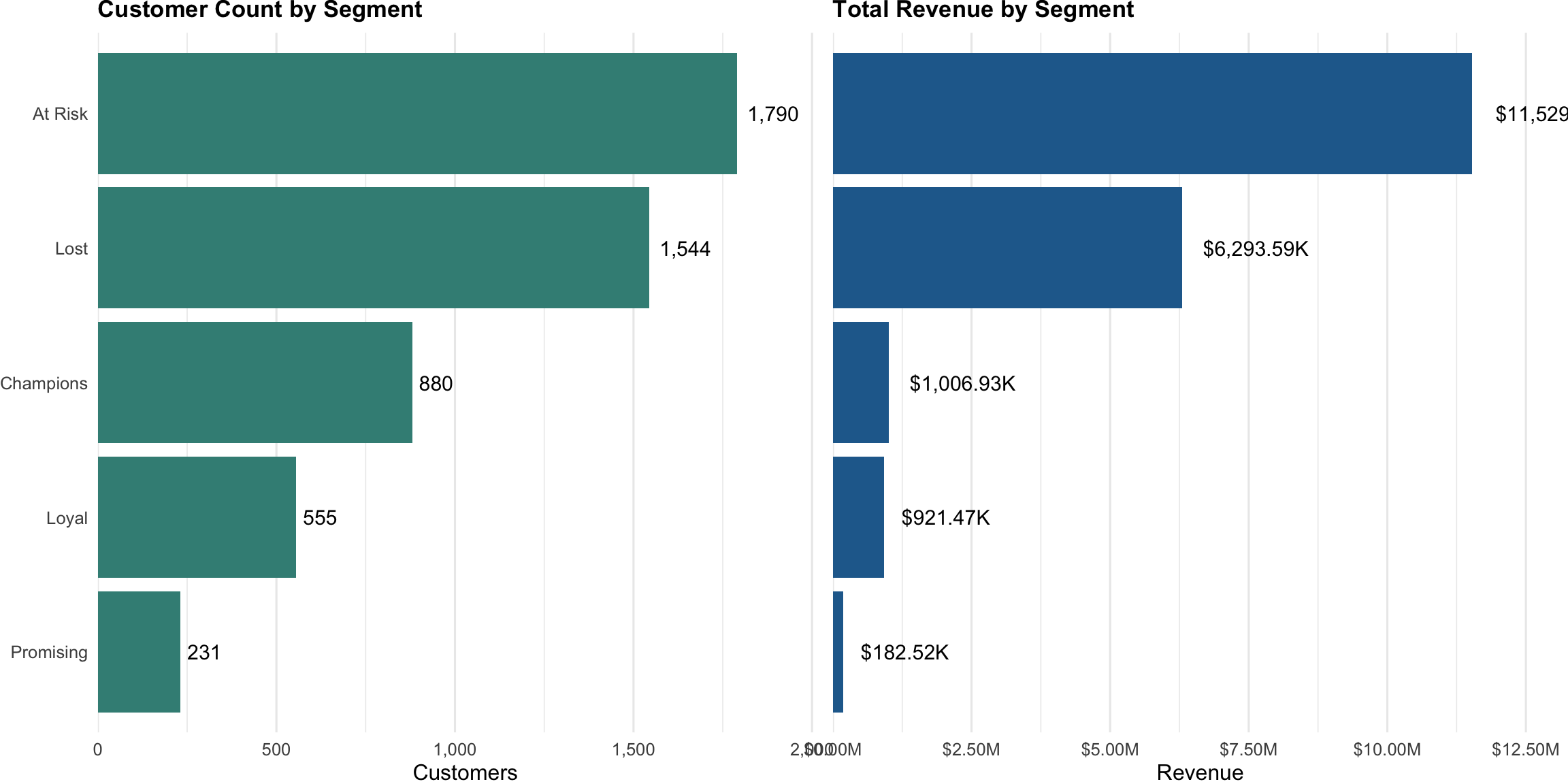
Segment profile analysis

Profiling segments by size, revenue contribution, and average metrics validates segmentation logic and informs resource allocation decisions.

RFM limitations

While powerful for segmentation, RFM has constraints that more sophisticated clustering techniques can address in advanced analysis.

What RFM Does Well

Simple, interpretable framework
Actionable segments with clear logic
Works with minimal data requirements
Business stakeholders understand it
Computationally efficient
Good baseline for many businesses

What RFM Misses

Arbitrarily groups continuous variables
Loses information in discretization
Can’t capture complex, non-linear patterns
Fixed rules may not fit all customers
Ignores product/category preferences
No statistical validation of segments
Misses velocity and trajectory nuances

Takeaway

RFM transforms individual metrics into strategic segments
Provides actionable framework for differentiated marketing
Foundation for understanding customer value and lifecycle
Starting point for more sophisticated analytical approaches