MKT 512 – Latent Variables and Factors

What is a Latent Variable?

Not directly observable or measurable
Exists as a construct combining multiple observable factors
Examples:
- Customer satisfaction
- Brand loyalty
- Purchase intention
- Product quality perception

Example

How satisifed are you with our service?

When is this sufficient?

Quick customer pulse checks
Transaction-specific feedback
Trend monitoring over time

When do we need more?

Understanding drivers of satisfaction
Predicting future behavior
Developing improvement strategies
Academic research requiring construct validity

Real-World Example: Customer Satisfaction

What are we really measuring?

Service quality?
Product performance?
Value perception?
Staff interaction?
Problem resolution?
Expectations vs. reality?
All of the above?

One question cannot usually capture this level of complexity.

Your turn

AI Prompt:
“Generate a set of 8-10 survey items to measure a consumer’s perception of a product’s relevance to
their life.”

Which items seem to measure different things? Can you name the possible dimensions they imply?
Are these items all measuring the same kind of relevance (e.g., personal, functional, social)?
Could two people read these items and interpret them differently based on their own experiences?

Multi-item scales

A multi-item scale is a measurement instrument that combines multiple related questions or items to assess a complex, underlying construct (latent variable) that cannot be directly observed or measured with a single question.

Key Features

Multiple related items measuring different aspects of the same construct
Increases reliability and validity compared to single-item measures
Reduces measurement error through item aggregation

Example

Customer satisfaction scale having multiple items to measure three distinct dimensions of satisfaction…

Contentment
Likelihood to recommend
Value for the money

When do we need scales?

Complex psychological constructs
(i.e, brand perception, purchase motivation, etc.)
Behavioral intentions
(i.e., likelihood to recommend, future purchase behavior, etc.)
Attitude measurement
(i.e., product preferences, service quality evaluation, etc.)

Benefits of well-designed scales

Increased reliability
Better construct validity
Reduced measurement error
Capture multiple dimensions
Enable factor analysis
Allow for internal consistency checks

Good example

Good design principles

Clear theoretical dimensions
Items that tap into the same construct but from different angles
Consistent level of abstraction
Items clearly relate to what we’re trying to measure
Items show good likelihood of internal consistency
Clear, simple language

Challenging example

A scale to measure environmental consciousness

I always recycle my plastic bottles
I think climate change is a serious issue
I enjoy spending time outdoors
I donate to environmental charities
I prefer natural scenery to city views

From scales to factors…

A galaxy is like a factor in the universe.

Factor analysis

Identify clusters of inter-correlated variables
Family of multivariate statistical techniques for exploring correlations between variables
Empirical approach to test theoretical data structures
Widely used method in psychometric instrument development

Purposes

Data reduction
Reduce number of variables in dataset to smaller set of factors
Theory development
Detect structural relationships between variables, often latent structures that describe a governing force

Theory development

Investigate underlying correlation patterns shared by variables in order to test a theoretical model (i.e. How many personality factors are there?)
Done well, always addresses a theoretical question
(rather than just calculating an arbirtrary factor score)

Factors in the wild

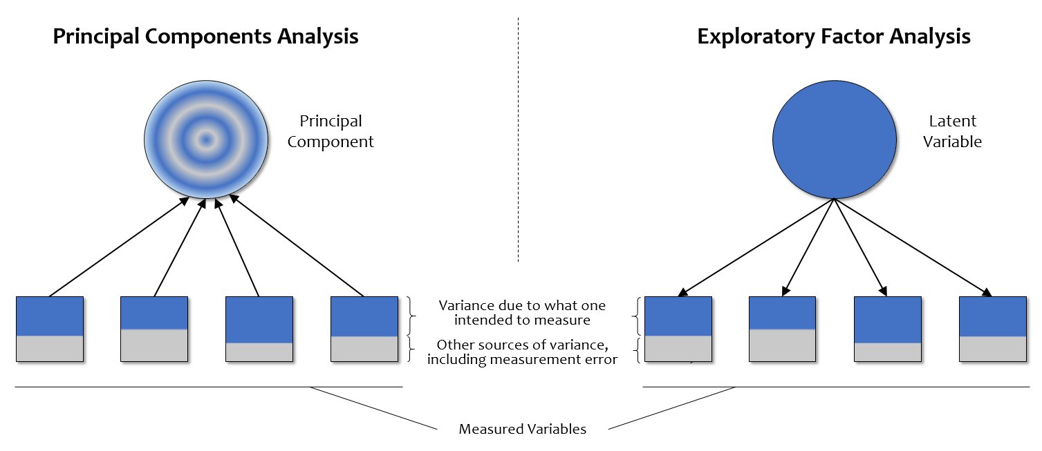
Approcahes to factor analysis

Principal Components Analysis (PCA)
A data reduction technique that summarizes variance in observed variables without assuming underlying latent constructs. Often used as a first step to explore structure and simplify data
Exploratory Factor Analysis (EFA)
Explore and summarize underlying correlational structure for a dataset
Confirmatory Factor Analysis (CFA)
Tests that a correlational structure, as hypothesized, exists in a dataset and measures “goodness of fit.”

Methods of data reduction

Principal Components Analysis (PCA)

For data reduction
Creates summary scores
Best for: Simplifying data, creating composite scores, reducing variables

Exploratory Factor Analysis (EFA)

For understanding underlying structures
Looks at shared patterns between variables
Best for: Theory development, scale development, understanding latent constructs

Differences

Assumptions

Garbage in; Garbage Out
Sample size matters
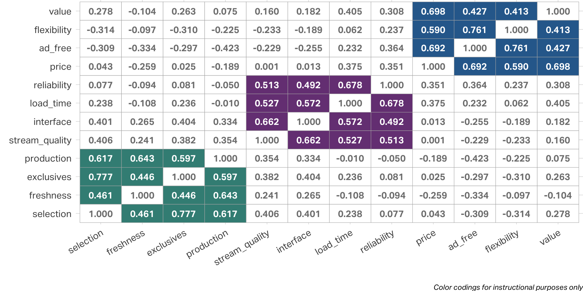
(Min = >5 cases per variable; Ideal = >20 cases per variable)
Interval or ratio data suitable for correlation analysis
Normality: normal distribution is ideal but not required
Outliers: Factor analysis is sensitive to outliers, which should be removed or transformed
Requires strong evidence of correlation
(correlation matrix coefficients > 0.3)

Process

Test assumptions
Select type of factor analysis
Determine number of factors
Select items
Name and define factors
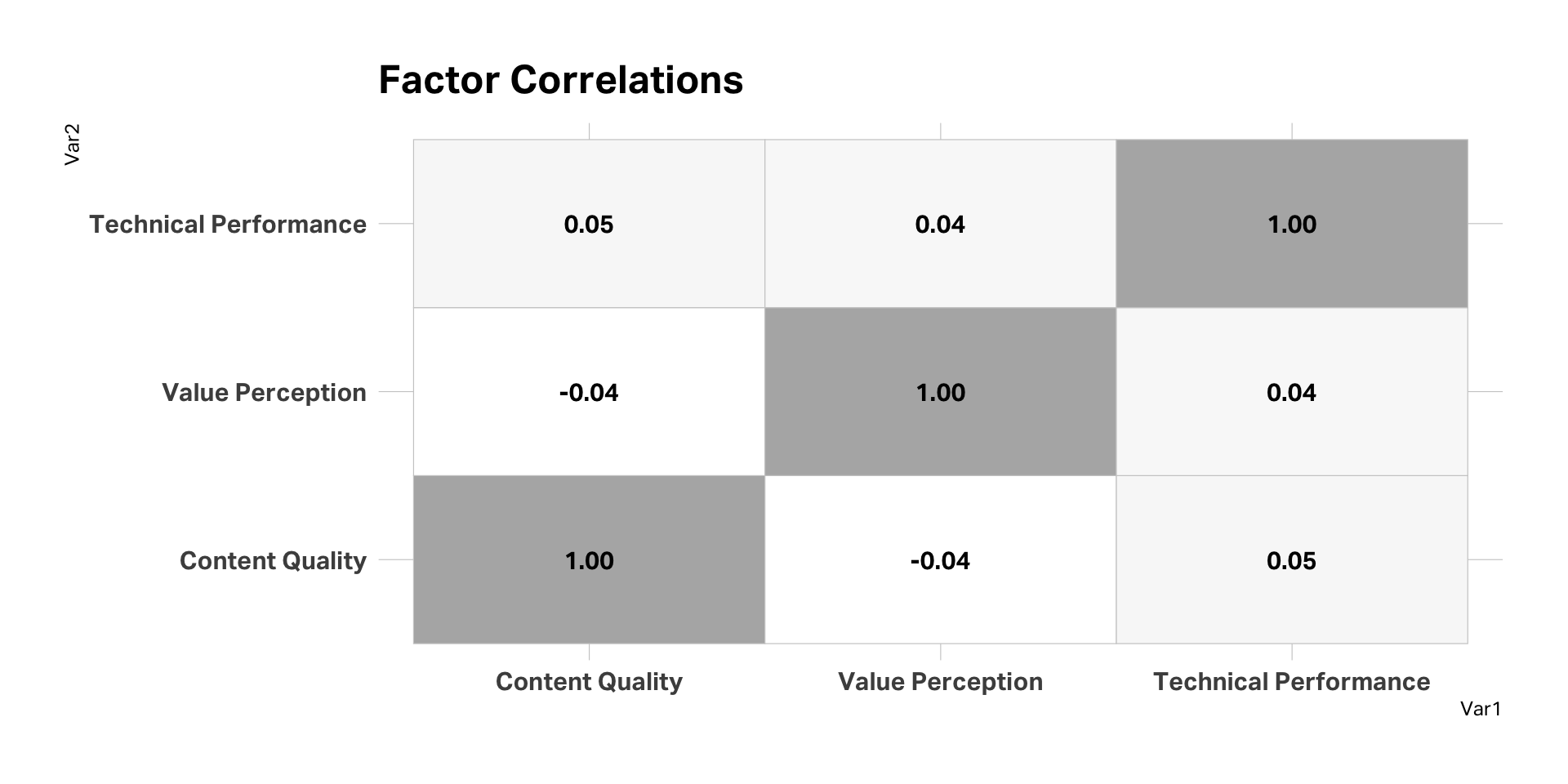
Examine correlations among factors
Analyze internal reliability
Compute composite scores

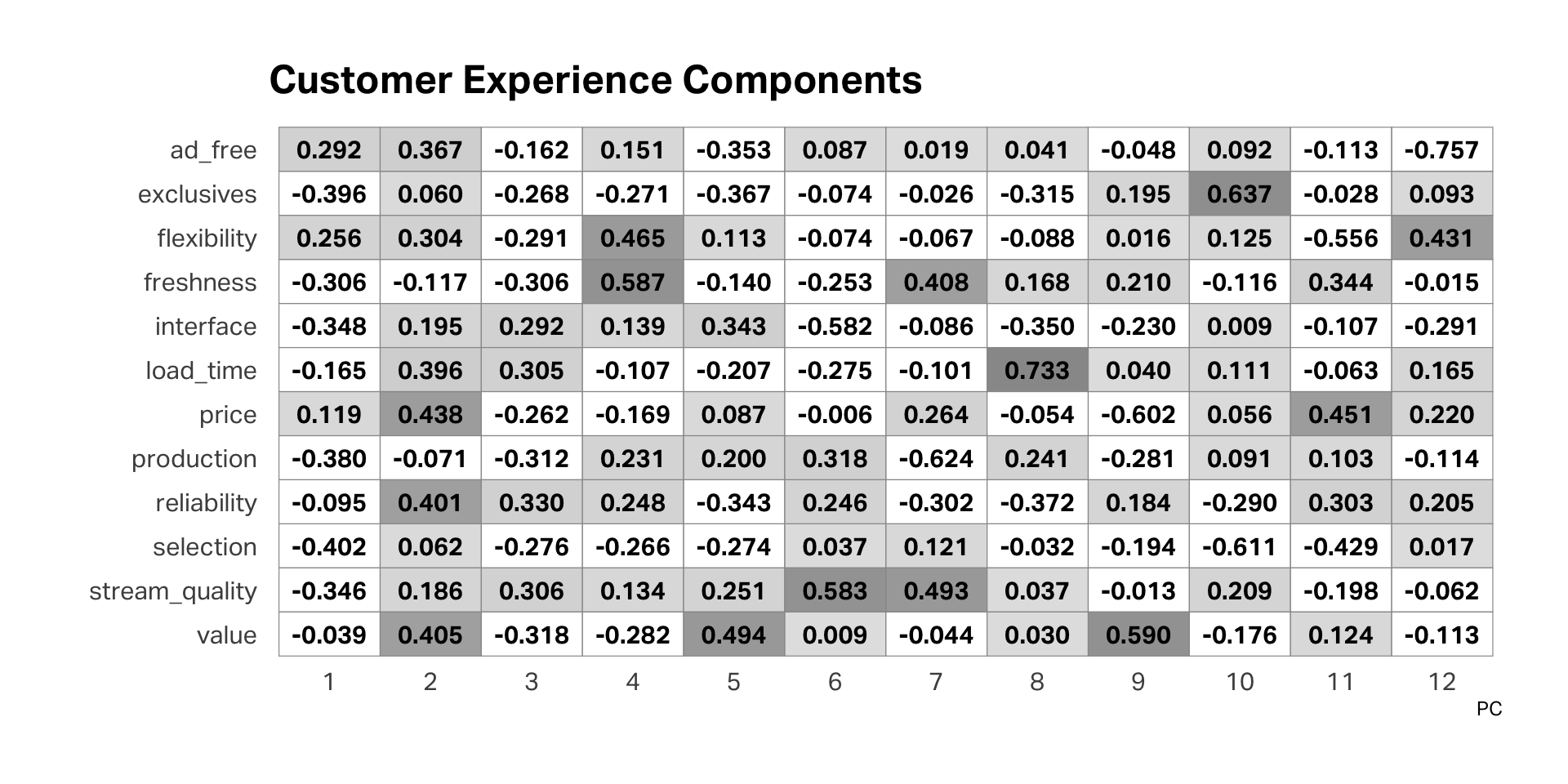
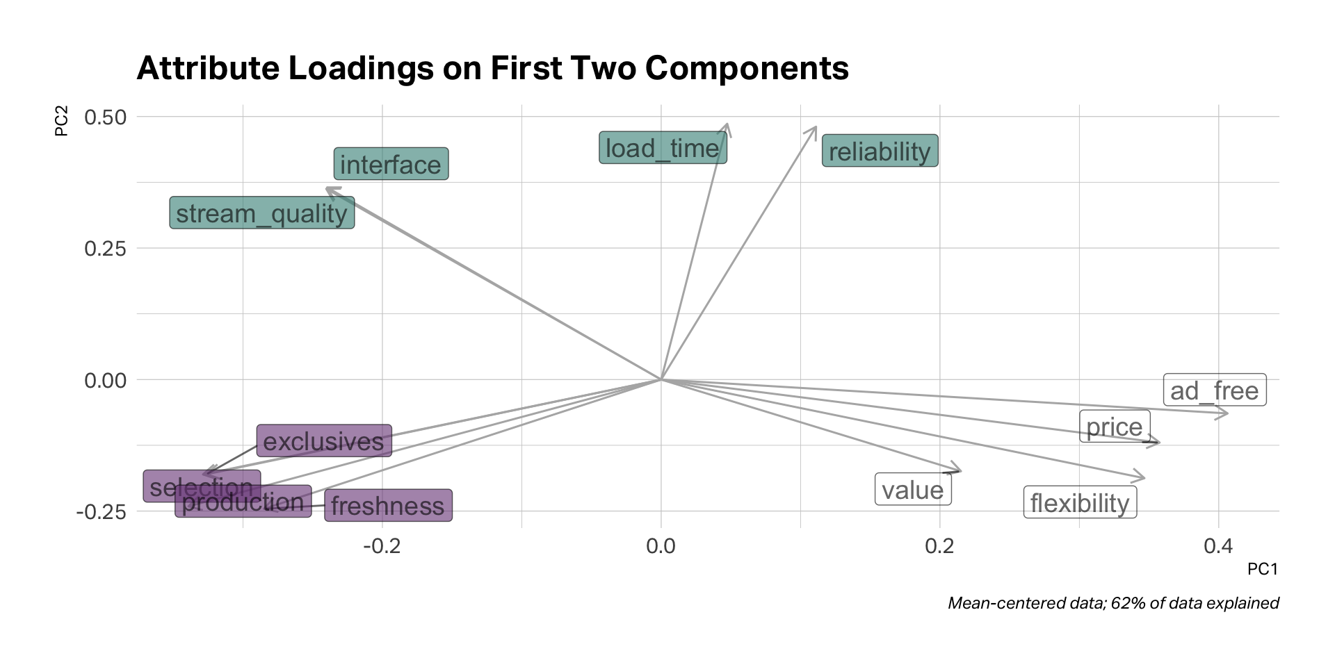
Customer experience dataset

variable	N	Median	Mean	SD	Min	Max
ad_free	515	4	3.61	1.85	1	7
exclusives	515	6	5.67	1.19	2	7
flexibility	515	4	3.97	1.49	1	7
freshness	515	5	5.36	1.15	2	7
interface	515	4	3.52	1.21	1	7
load_time	515	4	4.11	1.31	1	7
price	515	5	4.57	1.35	1	7
production	515	5	4.69	1.28	1	7
reliability	515	5	4.82	1.13	2	7
selection	515	5	4.79	1.35	1	7
stream_quality	515	5	4.53	1.20	1	7

Correlations

PCA

PCA in R

# Generate PCA data for the value attributes
atts_pca <- prcomp(atts, scale. = TRUE)

# Extract the component variables from the rotation matrix
atts_pca_tidy <- tidy(atts_pca, matrix = "rotation")

# Add the component data back to our original datafram for easy analysis
atts_pca_augment <- augment(atts_pca, atts)

PCA in R

# Generate PCA data for the value attributes
atts_pca <- prcomp(atts, scale. = TRUE)

# Extract the component variables from the rotation matrix
atts_pca_tidy <- tidy(atts_pca, matrix = "rotation")

# Add the component data back to our original datafram for easy analysis
atts_pca_augment <- augment(atts_pca, atts)

Rows: 515
Columns: 25
$ .rownames      <chr> "1", "2", "3", "4", "5", "6", "7", "8", "9", "10", "11"…
$ selection      <dbl> 5, 2, 4, 5, 4, 5, 4, 4, 4, 5, 5, 4, 5, 4, 4, 1, 3, 4, 4…
$ freshness      <dbl> 6, 4, 6, 6, 6, 6, 6, 5, 5, 6, 5, 5, 4, 6, 4, 2, 4, 5, 4…
$ exclusives     <dbl> 5, 5, 6, 6, 5, 7, 6, 7, 5, 6, 5, 5, 4, 5, 5, 2, 5, 5, 5…
$ production     <dbl> 6, 3, 3, 5, 4, 6, 5, 4, 4, 4, 2, 5, 4, 3, 4, 2, 4, 5, 5…
$ stream_quality <dbl> 5, 4, 3, 4, 3, 4, 5, 2, 3, 4, 2, 4, 3, 5, 3, 2, 4, 5, 5…
$ interface      <dbl> 4, 4, 3, 4, 2, 2, 3, 1, 1, 2, 1, 3, 3, 3, 2, 2, 3, 2, 2…
$ load_time      <dbl> 5, 4, 5, 6, 3, 3, 4, 1, 3, 3, 1, 4, 3, 3, 3, 3, 3, 4, 2…
$ reliability    <dbl> 6, 6, 5, 6, 5, 5, 5, 3, 4, 4, 2, 6, 4, 6, 4, 4, 5, 5, 6…
$ price          <dbl> 4, 6, 5, 4, 6, 4, 5, 5, 3, 4, 5, 5, 4, 6, 6, 4, 5, 5, 6…
$ ad_free        <dbl> 5, 6, 6, 5, 5, 5, 5, 5, 4, 5, 5, 5, 6, 6, 6, 4, 4, 4, 6…
$ flexibility    <dbl> 5, 7, 4, 5, 5, 5, 4, 5, 3, 5, 4, 5, 5, 6, 6, 4, 5, 4, 7…
$ value          <dbl> 5, 6, 5, 4, 4, 4, 5, 4, 4, 4, 4, 6, 5, 6, 6, 5, 5, 5, 6…
$ .fittedPC1     <dbl> -0.53921514, 2.83830534, 1.33551467, -0.38353822, 2.044…
$ .fittedPC2     <dbl> 0.97501116, 2.32547409, 0.63580098, 0.90671898, -0.2233…
$ .fittedPC3     <dbl> 0.198419179, 0.470935617, -0.223009414, 0.443588586, -0…
$ .fittedPC4     <dbl> 1.477343080, 0.708228129, -0.009214820, 1.098398190, 0.…
$ .fittedPC5     <dbl> -0.19965779, 0.61477373, -1.37297554, -1.42332925, -0.9…
$ .fittedPC6     <dbl> 0.31741410, -0.39843332, -1.13439459, -0.69495416, -0.0…
$ .fittedPC7     <dbl> -0.74490236, -0.31955883, 0.37527012, -0.73274202, 0.31…
$ .fittedPC8     <dbl> 0.49070944, -1.03674717, 0.28228210, 0.54056220, -0.237…
$ .fittedPC9     <dbl> 0.036735455, 0.313480138, 0.569294404, -0.004378656, -0…
$ .fittedPC10    <dbl> -0.43539543, 0.81600722, 0.25165611, 0.08061553, -0.176…
$ .fittedPC11    <dbl> -0.26016875, 0.02679340, 0.58930499, -0.34439566, 0.800…
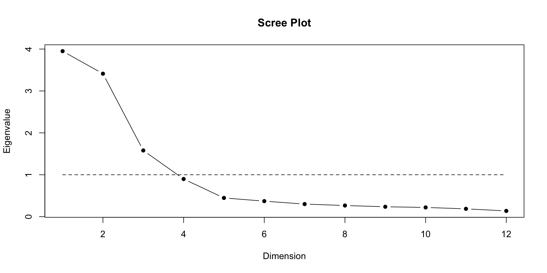
$ .fittedPC12    <dbl> -0.3488676821, 0.2388837178, -0.3910916532, 0.085246070…

PCA output

EFA

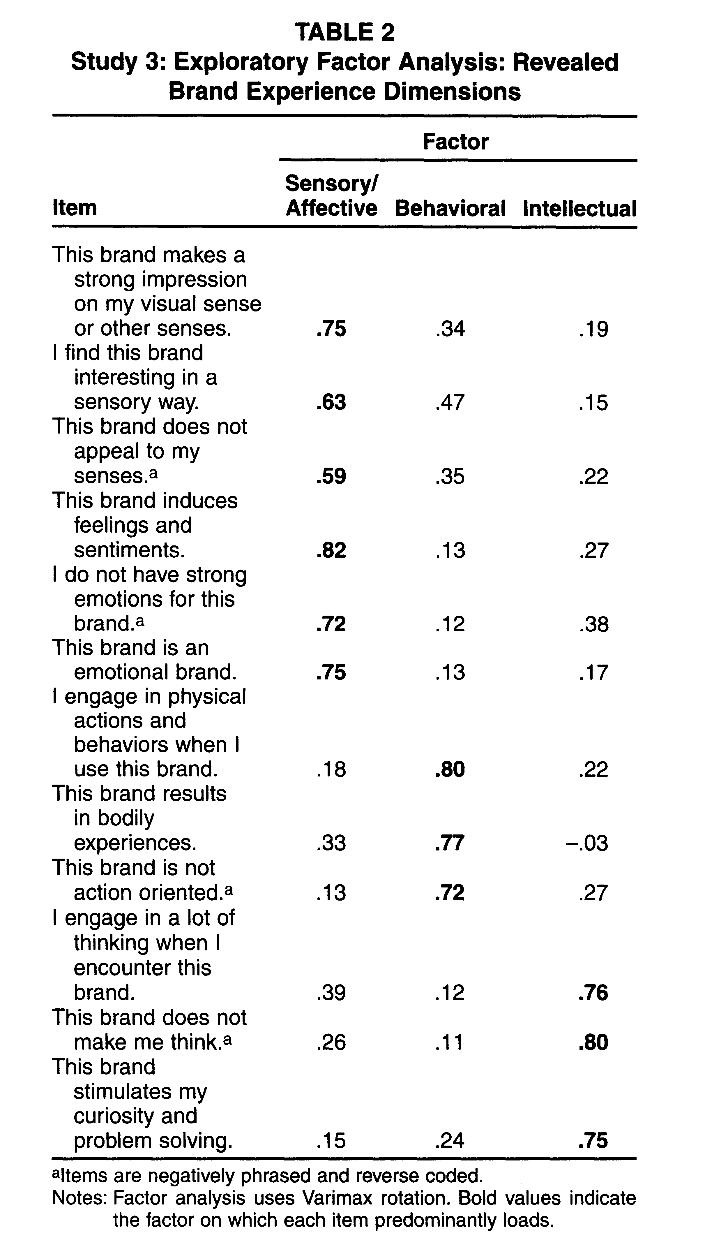
How many factors?

A good factor solution is one that explains the most variance with the fewest factors.

EFA statistics

n.factors	total.variance	statistic	p.value	df
1	0.258	2,770.311	0.000	54
2	0.529	1,291.999	0.000	43
3	0.662	507.220	0.000	33
4	0.733	154.632	0.000	24
5	0.762	29.974	0.018	16

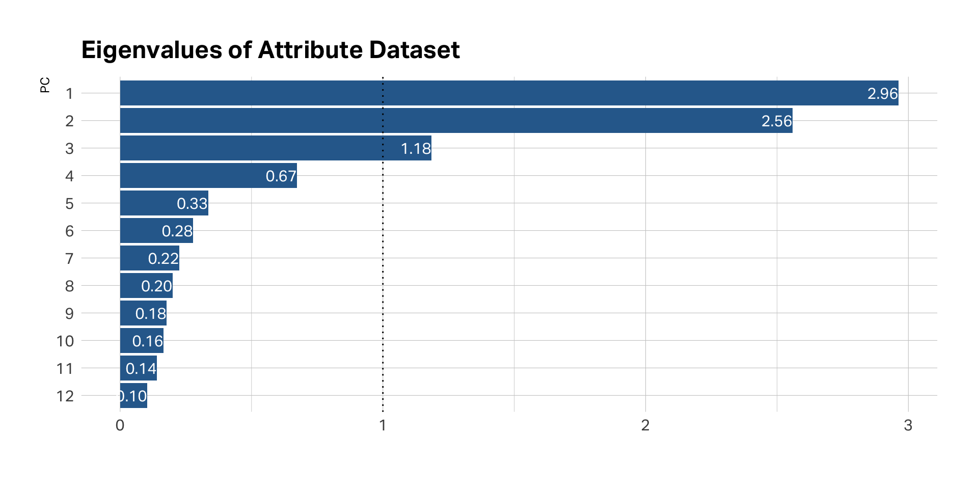
Eigen values

Each factor has an Eigen Value (EV) that indicates amount of variance it accounts for
EV for each successive factor has a lower value
Rule of thumb: EVs over 1 are “stable”

EVs on PCA

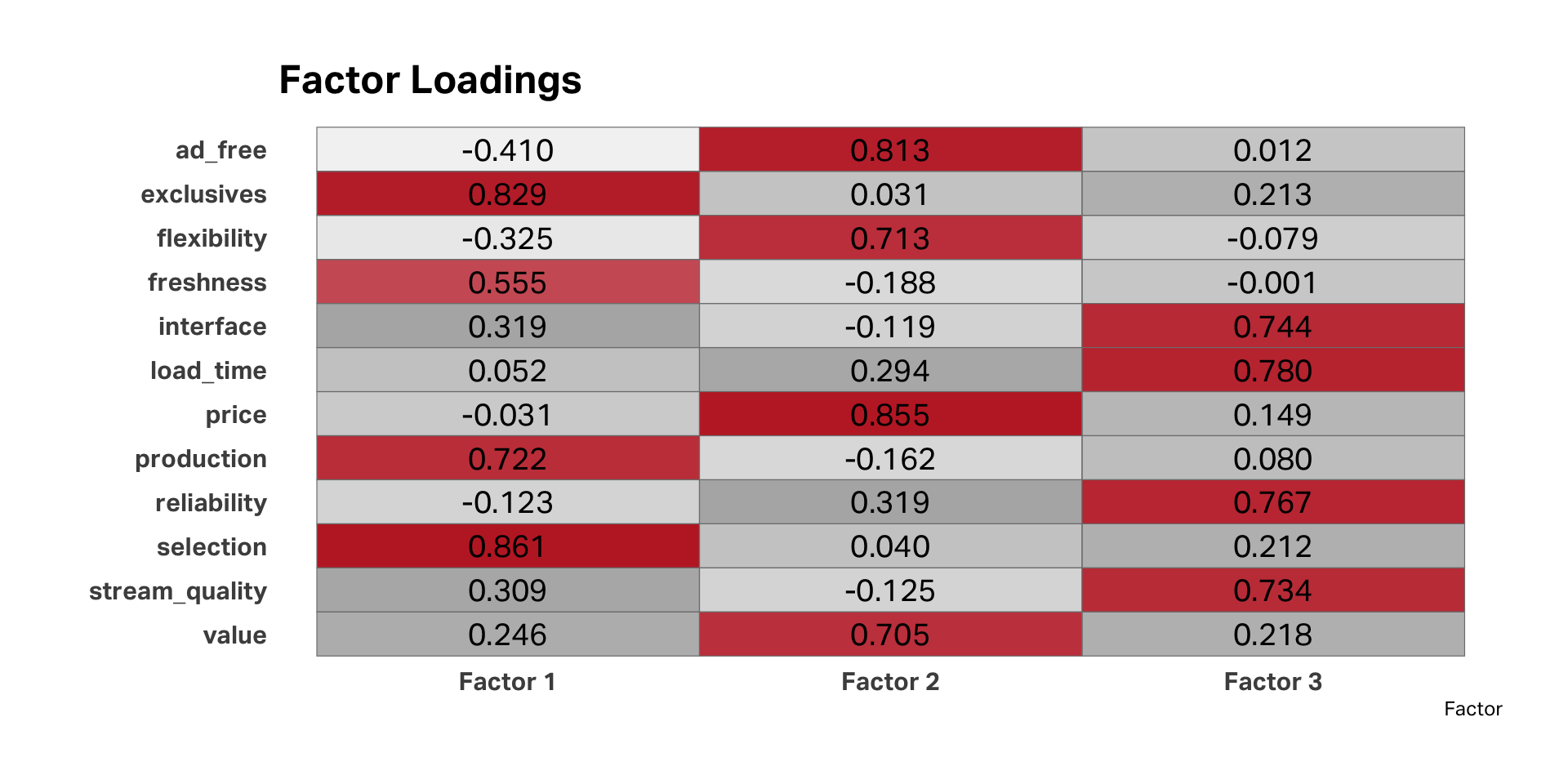
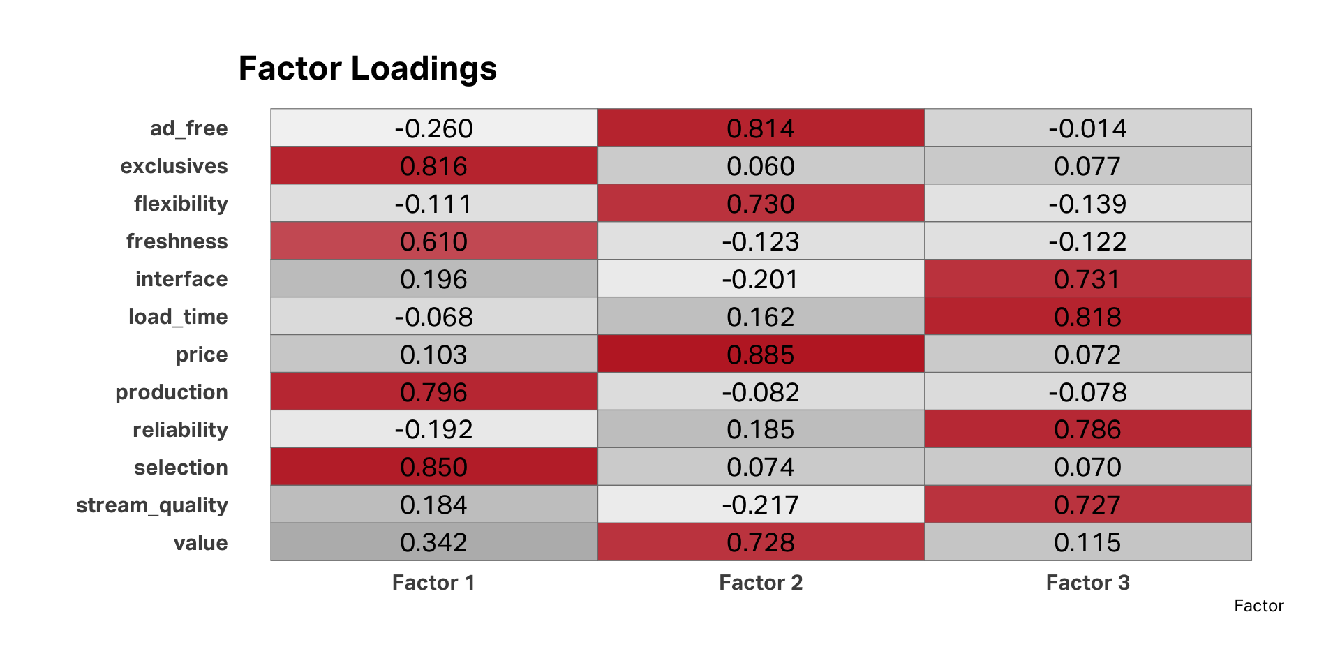
Factor loadings

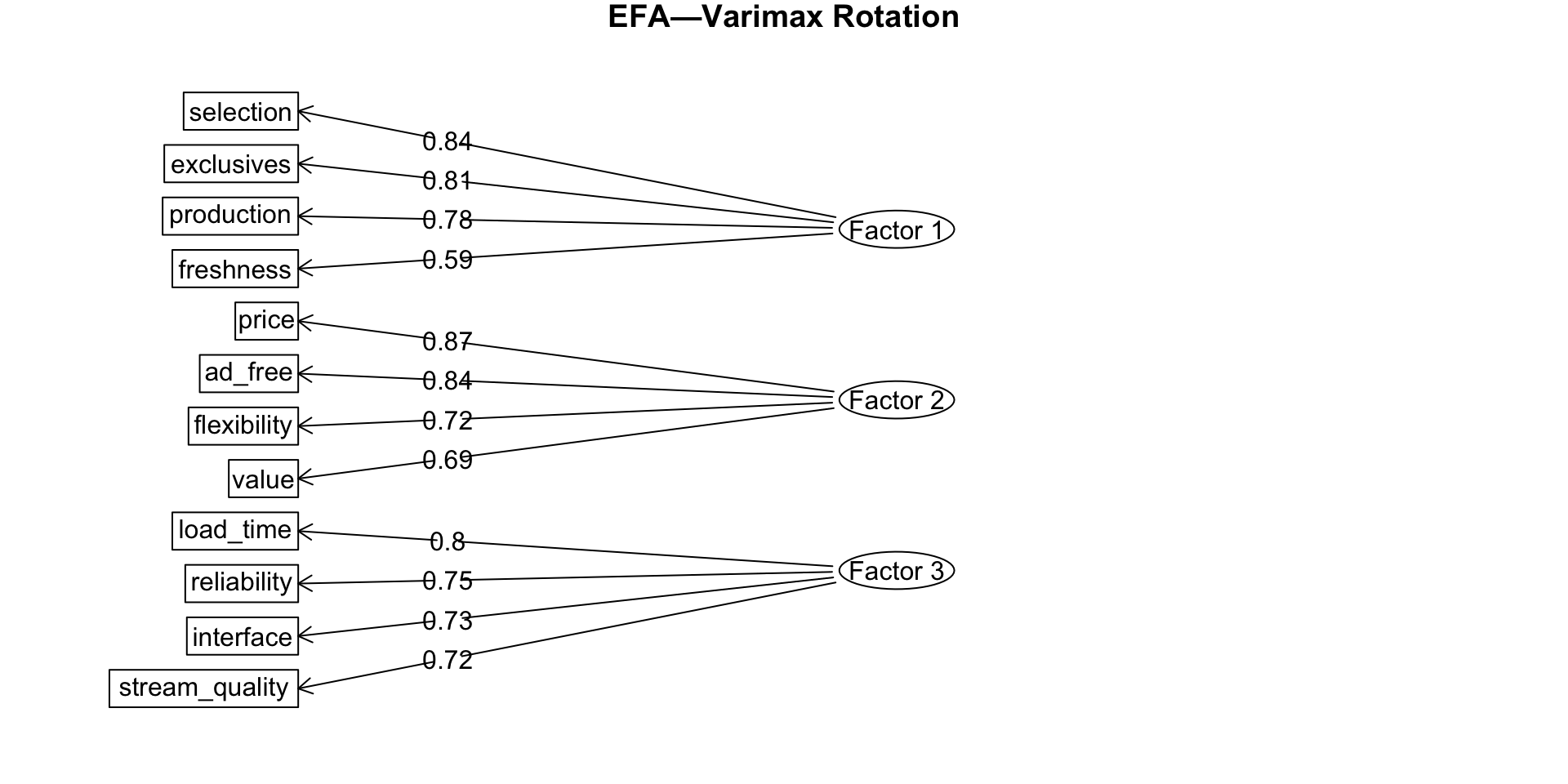
EFA diagram

Uniqueness

variable	uniqueness
freshness	0.656
production	0.446
value	0.395
flexibility	0.380
stream_quality	0.351
interface	0.330
load_time	0.303
reliability	0.295
exclusives	0.267
price	0.245
selection	0.212
ad_free	0.170

Rotation

Rotated factors

EFA diagram

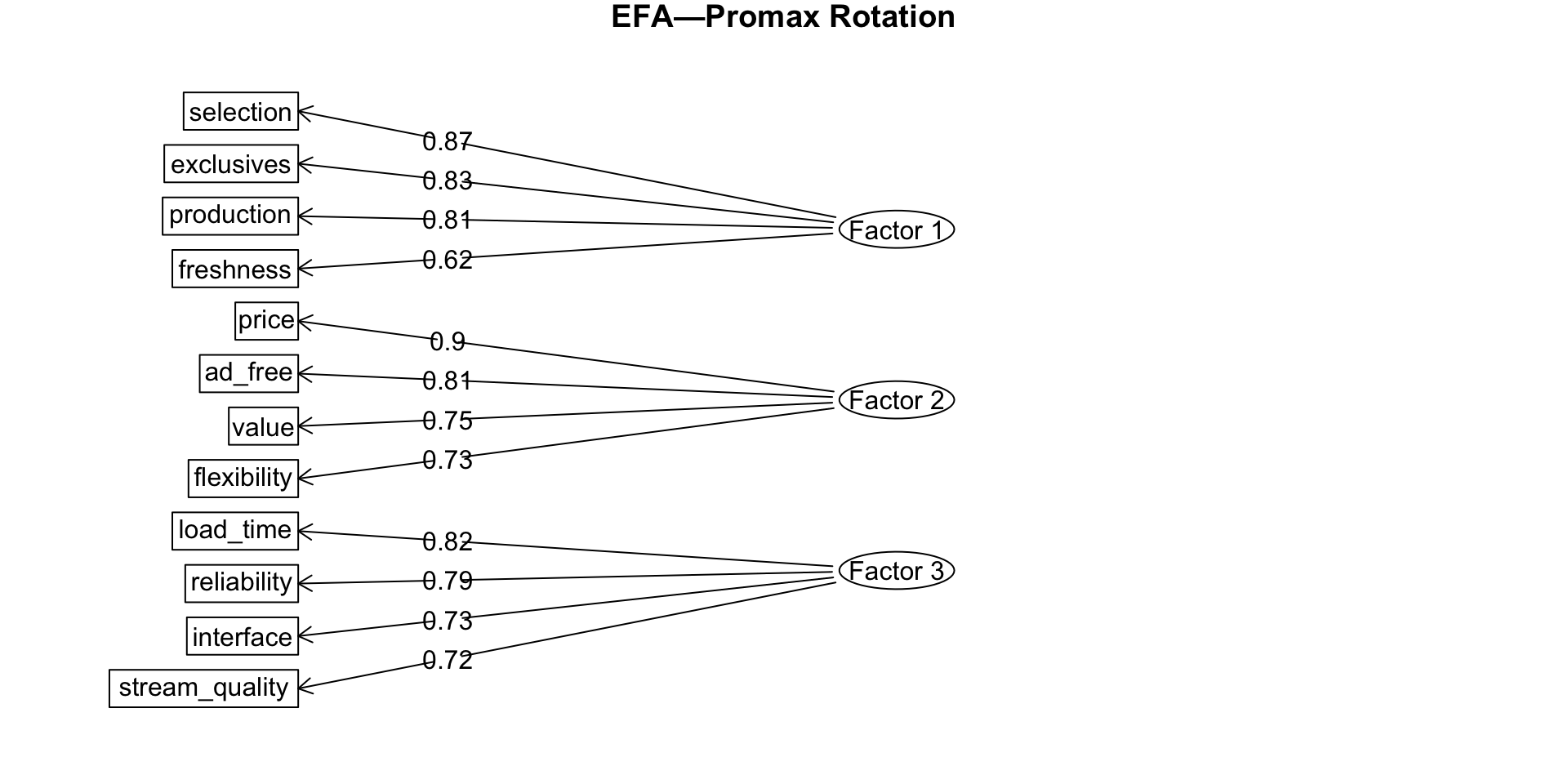
Naming the factors

Factor	Variables
Content Quality	Selection
	Freshness
	Exclusives
	Production Value
Technical Performance	Stream Quality
	Interface Ease
	Load Time
	Reliability
Value Perception	Price Fairness
	Ad Frequency
	Subscription Flexibility
	Overall Value

Check correlations

Determine reliability

Chronbach’s alpha is measure of internal reliability
Estimates how closely related a set of items are as a group
Alpha is assessed on a scale from 0-1

Alpha scores

factor	raw_alpha	std.alpha
Raw Alpha
Content	0.85	0.85
Technical	0.84	0.84
Value	0.85	0.86

variable	raw_alpha	std.alpha
Alpha Drops
Content
selection	0.79	0.79
freshness	0.85	0.86
exclusives	0.80	0.80
production	0.80	0.79
Technical
stream_quality	0.80	0.81
interface	0.80	0.80
load_time	0.79	0.79
reliability	0.81	0.81
Value
price	0.78	0.77
ad_free	0.79	0.80
flexibility	0.80	0.82
value	0.86	0.87

Composite scores

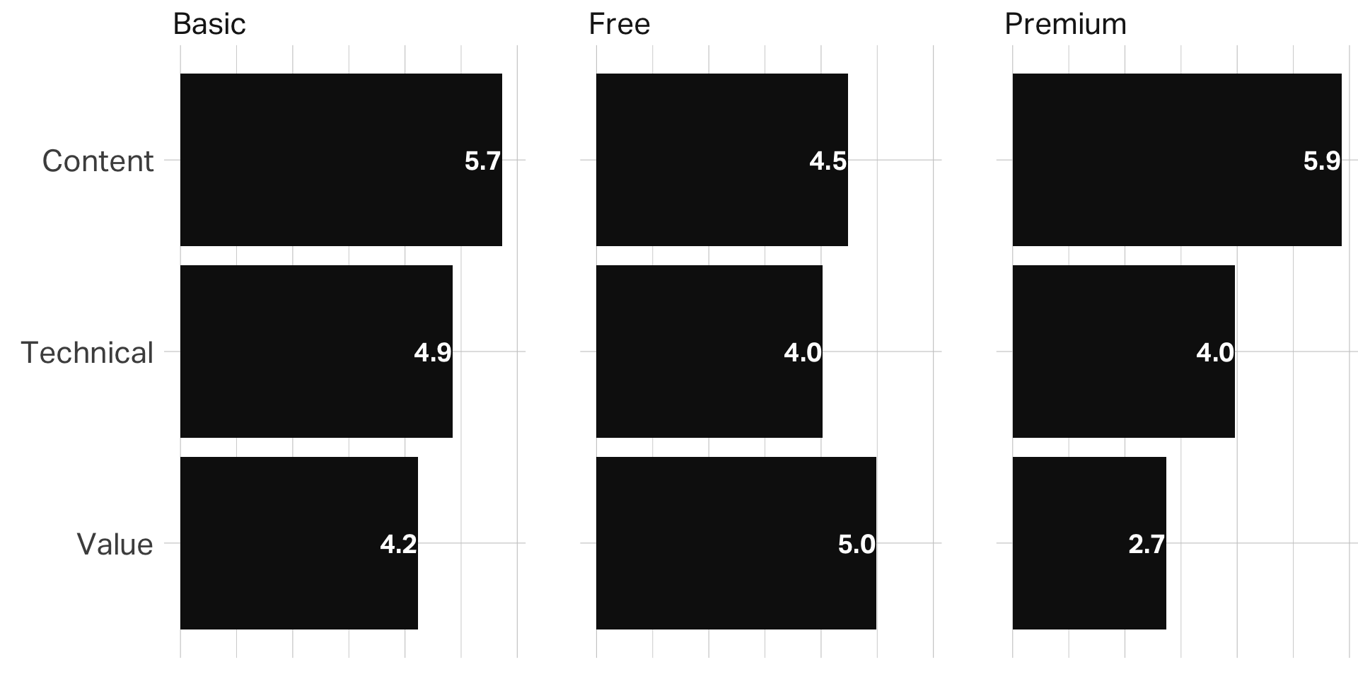
ANOVA

factor	contrast	estimate	conf.low	conf.high	adj.p.value
Content	Free-Basic	−1.3	−1.5	−1.1	0.00
Content	Premium-Basic	0.1	−0.1	0.4	0.45
Content	Premium-Free	1.4	1.2	1.6	0.00
Technical	Free-Basic	−0.8	−1.1	−0.6	0.00
Technical	Premium-Basic	−0.9	−1.2	−0.6	0.00
Technical	Premium-Free	−0.1	−0.3	0.2	0.82
Value	Free-Basic	0.7	0.5	1.0	0.00
Value	Premium-Basic	−1.5	−1.8	−1.2	0.00
Value	Premium-Free	−2.2	−2.5	−2.0	0.00

Latent Variables and Factors

Lecture

What is a Latent Variable?

Example

Real-World Example: Customer Satisfaction

One question cannot usually capture this level of complexity.

Your turn

Multi-item scales

When do we need scales?

Benefits of well-designed scales

Good example

Good design principles

Challenging example

From scales to factors…

A galaxy is like a factor in the universe.

Factor analysis

Purposes

Theory development

Factors in the wild

Approcahes to factor analysis

Methods of data reduction

Differences

Assumptions

Process

Customer experience dataset

Correlations

PCA

PCA in R

PCA in R

PCA output

EFA

How many factors?

A good factor solution is one that explains the most variance with the fewest factors.

EFA statistics

Eigen values

EVs on PCA

Factor loadings

EFA diagram

Uniqueness

Rotation

Rotated factors

EFA diagram

Naming the factors

Check correlations

Determine reliability

Alpha scores

Composite scores

ANOVA